Why Do Multiphase Simulations Take So Long?

This knowledge base article describes the reasons why multiphase analyses take so long to run, and also provides best practices to optimize the set up of multiphase simulations.

Courant Number

The reason behind the runtime of multiphase analysis is their transient nature. To allow you to optimize your simulation set up, first, we need to understand the limitations.

All transient analysis have their timestep size limited by the Courant-Friedrichs-Lewy condition, also known as CFL condition. For stability purposes, the CFL condition states that:

$$C = \frac{u\Delta t}{\Delta x} \le 1 \tag{1}$$

Where \(C\) is the Courant number, \(u\) is the local velocity at a given cell, \(\Delta t\) is the timestep size in seconds, and \(\Delta x\) is the local length between mesh elements.

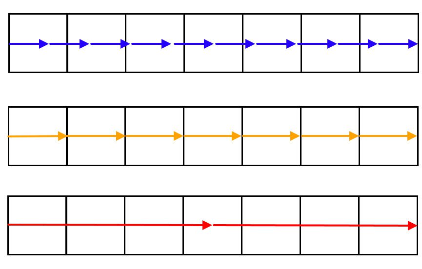
In Figure 1, you will find a visual representation of the CFL condition. Each square represents a mesh cell in the domain, and the arrows represent the distance traveled by a particle during a timestep. For the CFL condition to be satisfied, a particle should not completely skip a mesh cell during a timestep:

Therefore, the main objective of the setup of a multiphase analysis is to use large timestep sizes without having Courant numbers larger than 1.

Solution

Now that we know the requirements, what can we do in the simulation setup to satisfy them effectively? By inspecting equation 1, we observe that by using larger mesh cells, we can increase the timestep size while maintaining the Courant number under control.

In fact, crafting a very optimized and coarse hexahedral mesh is the most efficient way to increase the timestep sizes. Find below the best practices to run cost-effective multiphase analysis:

• Simplify the CAD model, removing small faces and details which won’t impact the results. Please visit this page for more details.
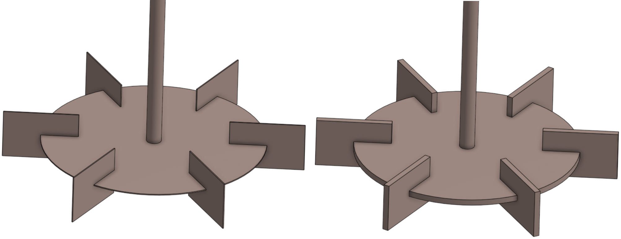
• If you have thin parts in your model, such as baffle walls or impellers, thicken them. This allows you to use coarser cells to capture the geometry

• Use a Hex-dominant (parametric) meshing tool to craft an optimized mesh for your geometry. This article provides insights about meshes for multiphase analysis.
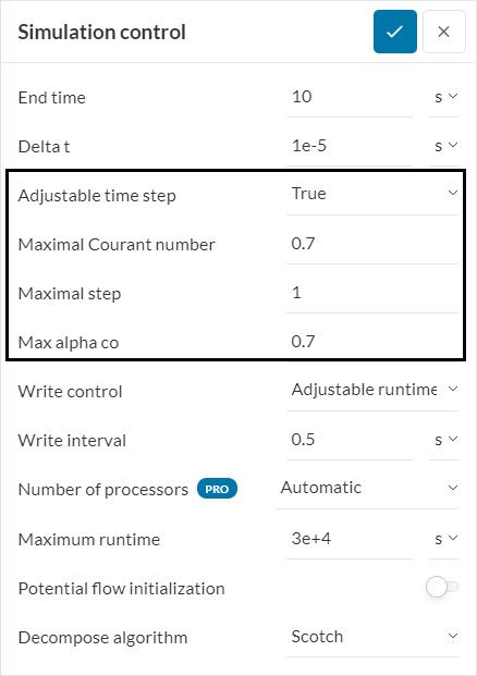
• Under the Simulation control settings, make sure that the Adjustable time step is set to True. This way, the algorithm will automatically adjust the timestep size to satisfy the Maximal Courant number that was defined.
  
  Furthermore, defining 0.7 to Maximal Courant number and Max alpha co is a good compromise between runtime and stability. For more notes on the purpose of each simulation control setting, please visit this page.

• Lastly, using equation 1, estimate the timestep size of each iteration. With this number in mind, set a sensible value for the End time of the simulation, remembering that each iteration takes time to calculate.