How to Obtain Heat Fluxes and Heat Transfer Coefficients from the Simulation Results?

In CFD simulations involving heat transfer, users are often interested in obtaining the heat flux and heat transfer coefficients from the simulation results, so they can assess and improve their designs from a thermal management perspective.

This article will explore the workflows available in SimScale to obtain the heat fluxes and heat transfer coefficients.

Overview

The heat transfer coefficient, denoted by $h$, can be an important design parameter for applications involving convective heat fluxes. The general formulation is given by Newton’s law of cooling:

$$\begin{array}{}\text{(1)}& q=hA(T_{wall}-T_{reference})\end{array}$$

Where:

• $q$ is the heat flux through the boundary, in $W$
• $h$ is the heat transfer coefficient, in $\frac{W}{m^{2}K}$
• $A$ is the surface area at which the heat transfer takes place, in $m^2$
• $T_{wall}$ is the temperature at the wall, in $K$
• $T_{reference}$ is a temperature of reference, in $K$

During any CFD simulation involving heat transfer, the values of $q$ and $T_{wall}$ are calculated by the solver for each iteration. Since the solver knows the areas of the surfaces, this leaves a single unknown left to obtain the heat transfer coefficient: $T_{reference}$.

There are two possibilities to determine $T_{reference}$, which will be explored in the next section.

Heat Transfer Coefficients Using Result Control

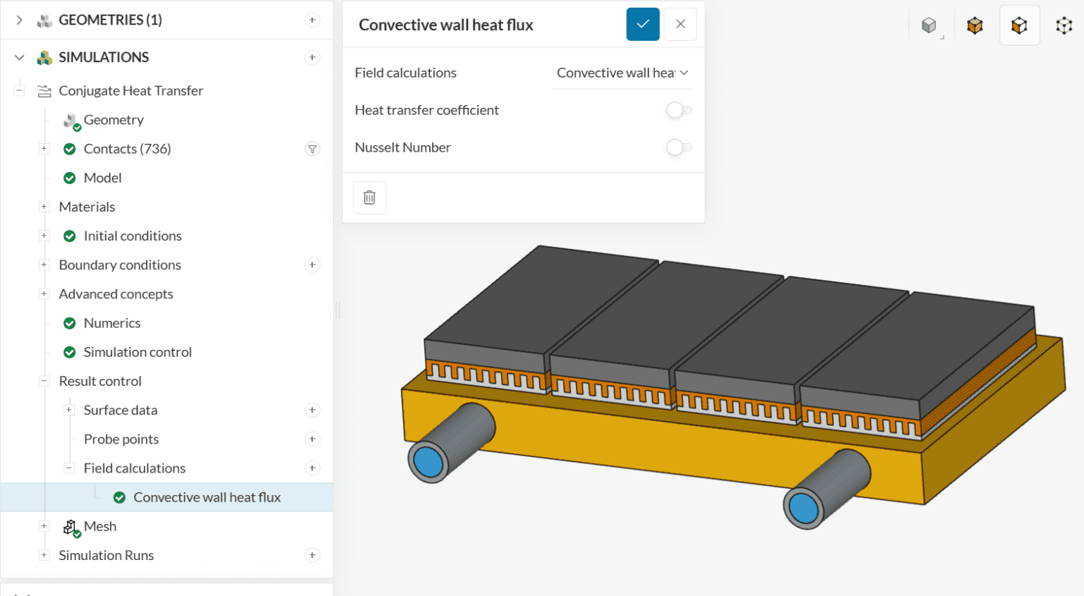
In SimScale, to obtain numerical results for the heat transfer coefficient, the user needs to set a result control before running the simulation:

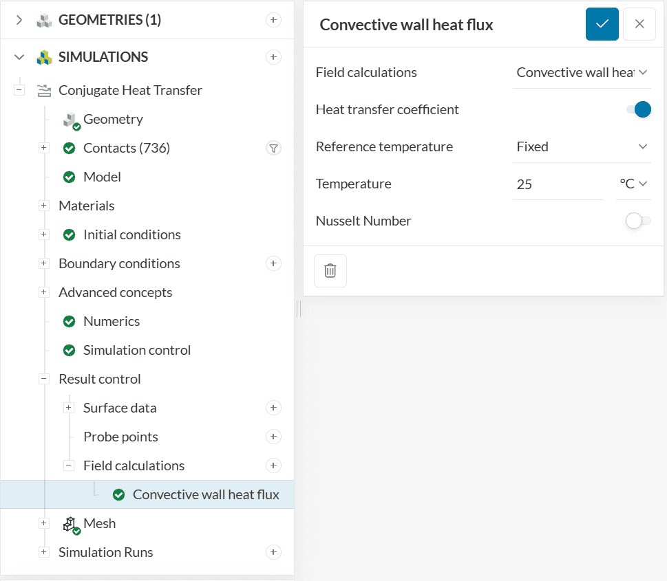
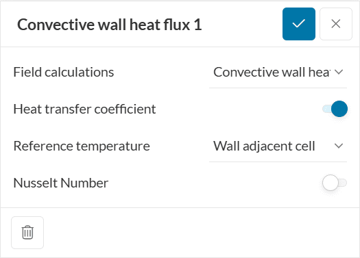
The Heat transfer coefficient toggle is available under the Convective wall heat flux result control, within Field calculations. When Heat transfer coefficient is active, the user has two options to define the Reference temperature ($T_{reference}$ from equation 1):

• Wall adjacent cell: This approach uses the temperature at the centroid of the first cell off the wall as the reference temperature
• Fixed: With this approach, the user specifies a representative reference temperature for their case

An overview of the available methods is provided below.

Wall Adjacent Cell

By using the Wall Adjacent Cell approach, SimScale uses the temperature on the centroid of the first cell away from the wall as $T_{reference}$ for the heat transfer coefficient calculation.

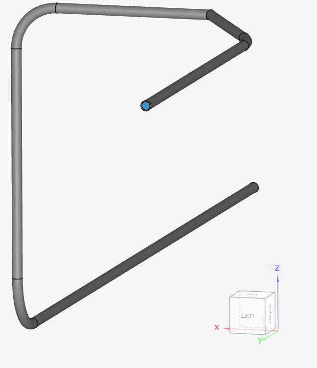
For illustrative purposes, let’s consider the following internal pipe flow simulation:

The mesh used in this sample case has 3 boundary layers. On a cell-by-cell basis, the algorithm determines the temperature of the centroid of the first cell away from the wall. In this particular example, the first cell will always be the first boundary layer:

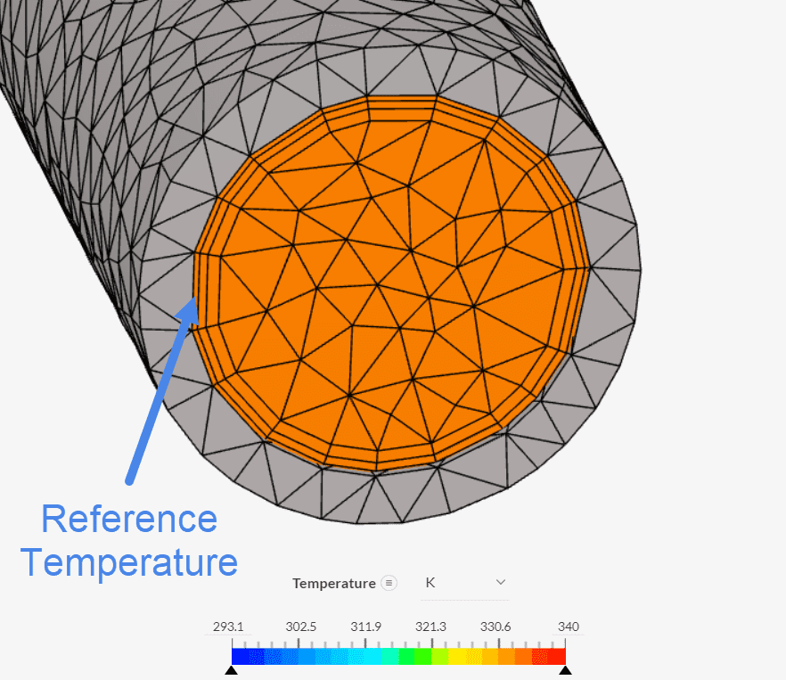
This approach is fairly automated, however, it also has a downside: the reference temperature is impacted by the mesh. If a different mesh had been used, the temperature of the first layer would likely be different due to the near-wall treatment. As such, different meshes may show different results for the heat transfer coefficient, even though the flow conditions remain the same.

Fixed Temperature

The Fixed temperature method is an alternative approach to setting a reference temperature, but less prone to mesh effects. In the configuration window, the user specifies the reference temperature directly, which is kept constant in the calculation.

Since the definition of the reference temperature solely depends on the user, caution needs to be exercised to define a representative value.

As an example, let’s consider a thermal management application where an enclosure is surrounded by air. The objective is to determine the heat transfer coefficient between the external walls of the case and the surrounding environment.

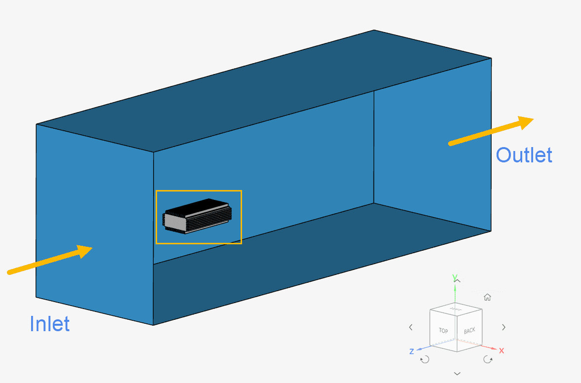
In this example, air enters the domain at 2 meters per second and 298.15 Kelvin. For external flow cases, the inlet temperature is a common choice for $T_{reference}$.

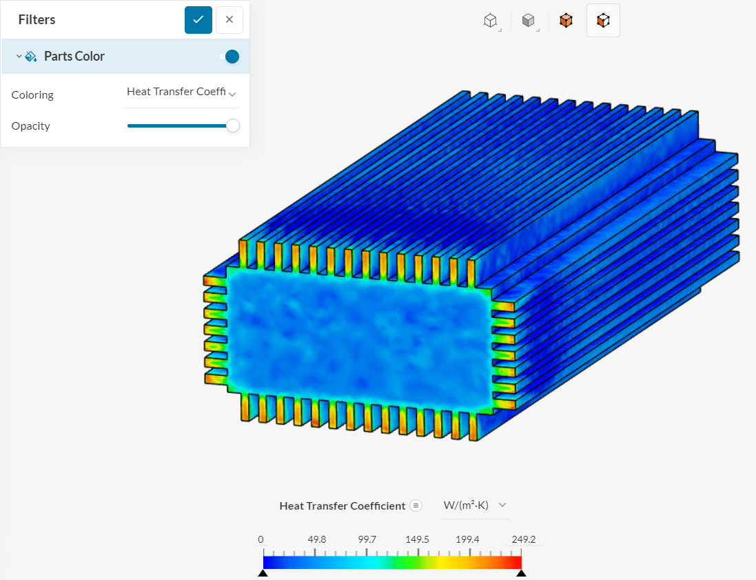
After running the analysis, you will receive the heat transfer coefficients on the fluid boundaries:

For internal flow cases, weighted averages of temperature or other strategies can be used to determine the reference temperature.

Heat Transfer Coefficients Using Field Calculator

In some cases, it can be useful to analyze different regions of the domain with different reference temperatures. Instead of running multiple result controls with different temperatures, users can take advantage of the Field Calculator filter, and input the heat transfer coefficient formula manually:

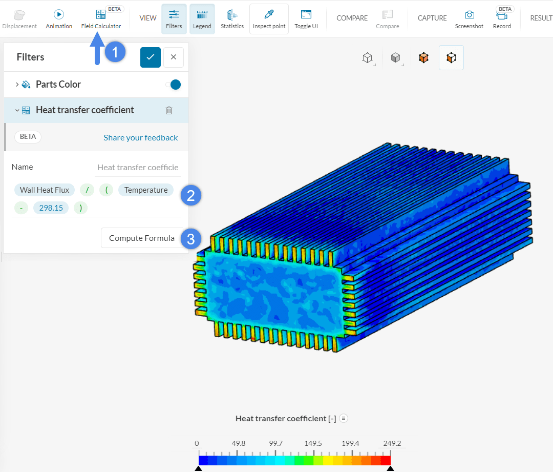
1. Create a Field Calculator entry
2. Set the formula of interest and the name of the new field
3. Compute the formula

As a reminder, the wall heat flux is in $\frac{W}{m^2}$ in the post-processor, therefore the formula is the following:

$$\begin{array}{}\text{(2)}& h=\frac{WallHeatFlux}{Temperature–T_{ref}}\end{array}$$

Obtaining Heat Fluxes in SimScale

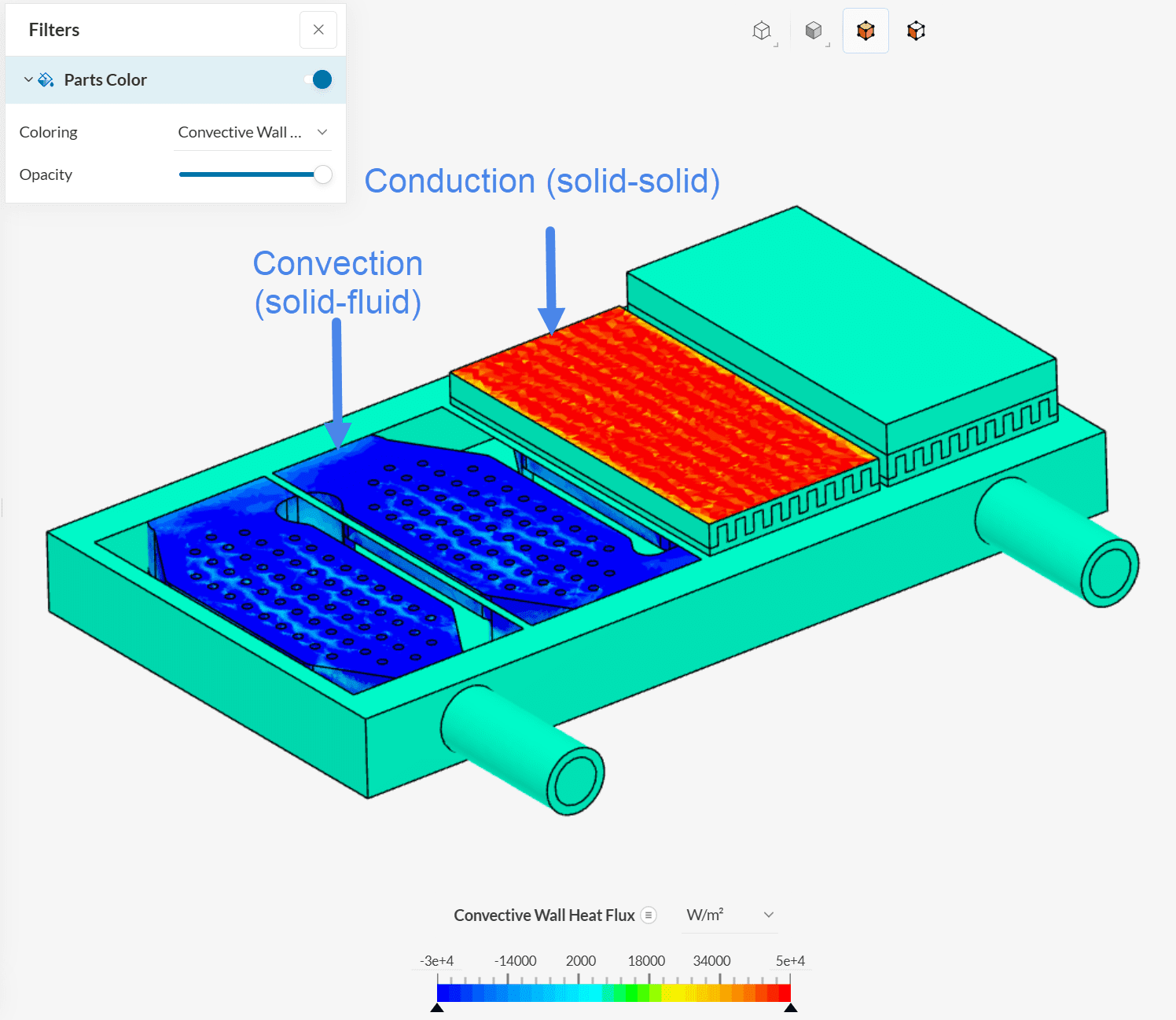
As discussed above, in Conjugate Heat Transfer simulations, heat fluxes are displayed in the post-processor if the user sets a Convective wall heat flux result control before launching the simulation.

More precisely, this result control shows heat fluxes due to convection and conduction. That is, you may see values for heat flux on all non-adiabatic walls of the computational domain, as conduction or convection may occur.

For example, taking a Conjugate Heat Transfer v2.0 simulation using the cold plate from Figure 8, we can observe convective heat fluxes between water and the cold plate in the post-processor, as well as heat fluxes due to conduction on the interfaces of the chips.

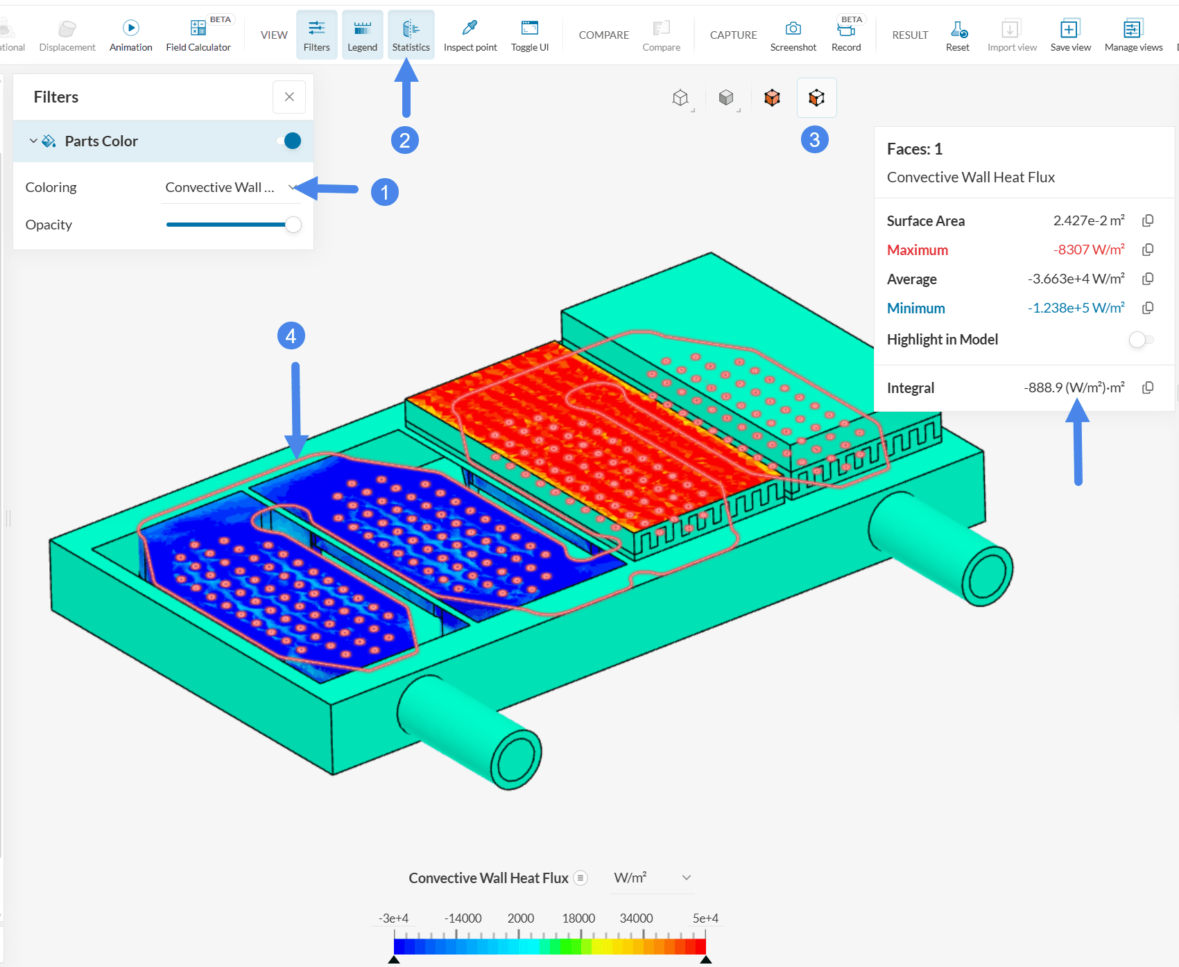
By using Statistics and selecting faces of interest, you can obtain heat fluxes through them:

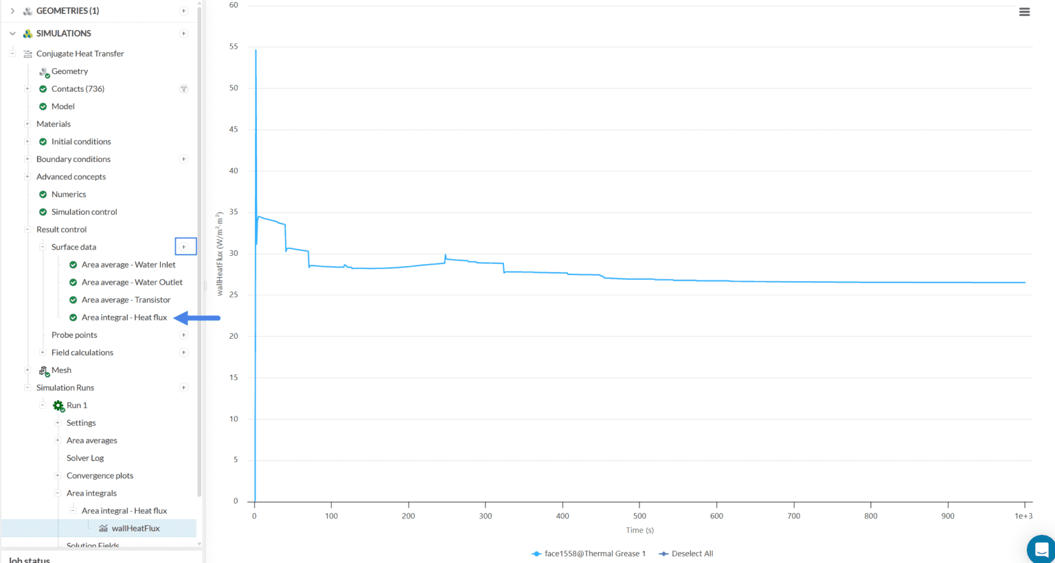
If you want to readily obtain heat fluxes due to conduction or convection on a certain face of interest without using the post-processor, a good workflow is to define an Area integral result control to that face.

Net Radiative Heat Fluxes

Note that, for simulations with radiation enabled, the Convective wall heat flux field in the post-processor does not account for radiation.

Instead, radiation has its own field in the post-processor, called Net radiative heat flux:

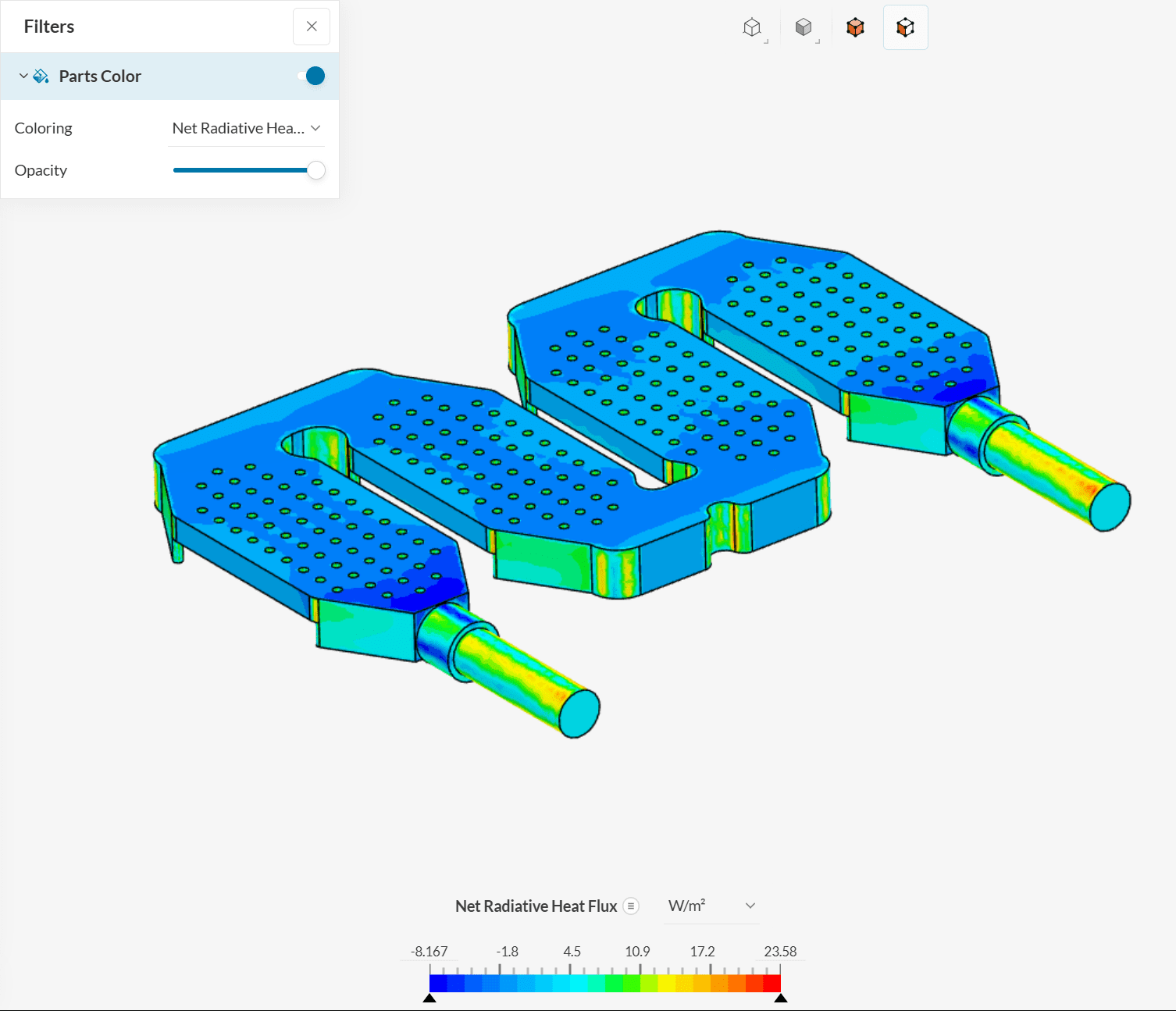
This field presents you with the net effects of radiation on a surface. That means, it is the summation of the amount of heat absorbed minus the amount of heat emitted via radiation by the surface.

All simulations involving radiation automatically generate a Net radiative heat flux result in the post-processor, therefore this does not require additional configurations by the user.