How to Model the Ground Roughness in Incompressible Analysis?

This article explains the best practices for modelling the ground roughness in SimScale’s incompressible flow simulation, which can also be applied to other simulations. For example, a convective heat transfer or conjugate heat transfer analysis.

One of the most influencing factors in an external aerodynamic simulation is ground roughness, therefore it is can be important to model the ground roughness in a CFD simulation.

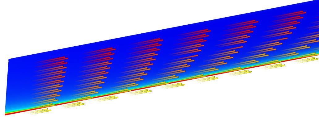
A Fully Developed ABL Profile

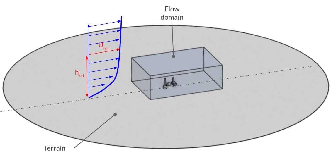
Atmospheric Boundary Layer (ABL) is a model to explain the earth’s lower atmosphere and its behaviour with respect to the ground. On the other hand, the velocity (\(u\)) profile is assumed to be logarithmic and turbulent kinetic energy (\(k\)) and turbulent dissipation rate \(\varepsilon\) are height dependent.

Moreover, if you need more information regarding how to calculate ABL profile, please visit this knowledge base article.

Sand-Grain Roughness Modification

The incompressible flow simulation solver implemented in SimScale uses wall functions as default. Hence, the rough wall function model uses equivalent sand-grain roughness (\(k_s\)) and roughness constant (\(C_s\)) parameters.

This wall function is originally developed for pipe flows, therefore the aerodynamic roughness length (\(z_0\)) should be modified for equivalent roughness. Likewise, a good approximation for an equivalent sand-grain roughness takes both the terrain aerodynamic roughness length and a roughness constant into account which can be expressed with the equation below:

$$k_s = \frac{9.793 \cdot z_0}{C_s} \tag{1}$$

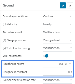
In the following table, you will see the mean terrain roughness length (\(z_0\)) per terrain class, and corresponding roughness length (\(k_s\)) and minimum first cell height requirements in CFD modeling. Cell size values are calculated for roughness constant of 1 (\(C_s\)), but you can multiply the height by 2 if you need to use roughness constant of 0.5. [1]

Terrain Class	mean \(z_0\) [m]	\(k_s\) [m]	\(C_s\)	h [m]
1	0.0001	0.001	1	0.002
2	0.0005	0.0049	1	0.01
3	0.005	0.049	1	0.1
4	0.03	0.2938	1	0.6
5	0.07	0.6855	1	1.4
6	0.55	5.3862	1	10.8
7	2.5	24.4825	1	49

Basic Recommendations for an Accurate ABL Profile

However, an accurate representation of ABL profile on the near ground regions may be challenging to achieve in CFD, therefore there are many studies on how to achieve the most accurate results. For example, a study from Blocken et al. [2] suggested the following measures to capture the ABL profile as close as possible:

1. Firstly, You need a high mesh resolution around the ground level. A minimum of 2 or 3 elements (or layers) is required for pedestrian wind comfort simulations. In general, keep the first cell height less than 1 \(m\).

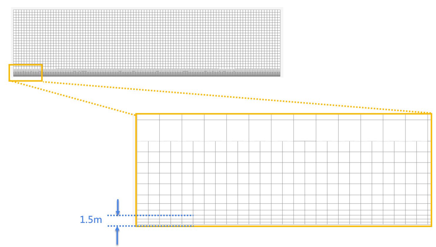
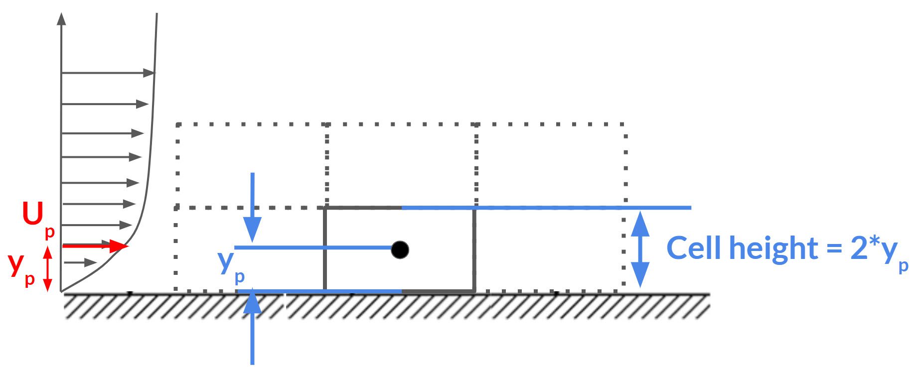
2. Keep the height of the center point \(y_p\) of the first cell (or layer) larger than the equivalent sand grain roughness height \(k_s\) (\(y_p\)>\(k_s\)).

3. Lastly, make sure that the ABL profile is homogeneous from the upstream to the downstream.

4. And then you can find a good approximation regarding the relationship between the \(k_s\) and \(z_0\).

References

- Toparlar, Y., Blocken, B., & Van Heijst, G.(2019). “CFD Simulation of the Near-neutral Atmospheric Boundary Layer: New Temperature Inlet Profile Consistent with Wall Functions”. Journal of Wind Engineering and Industrial Aerodynamics, 191, 91-102.https://doi.org/10.1016/j.jweia.2019.05.016
- Blocken, B., Stathopoulos, T., & Carmeliet, J. (2007). “CFD simulation of the Atmospheric Boundary Layer: Wall Function Problems”. Atmospheric Environment, 41(2), 238-52.https://doi.org/10.1016/j.atmosenv.2006.08.019
Note
If none of the above suggestions solved your problem, then please post the issue on our forum or contact us.