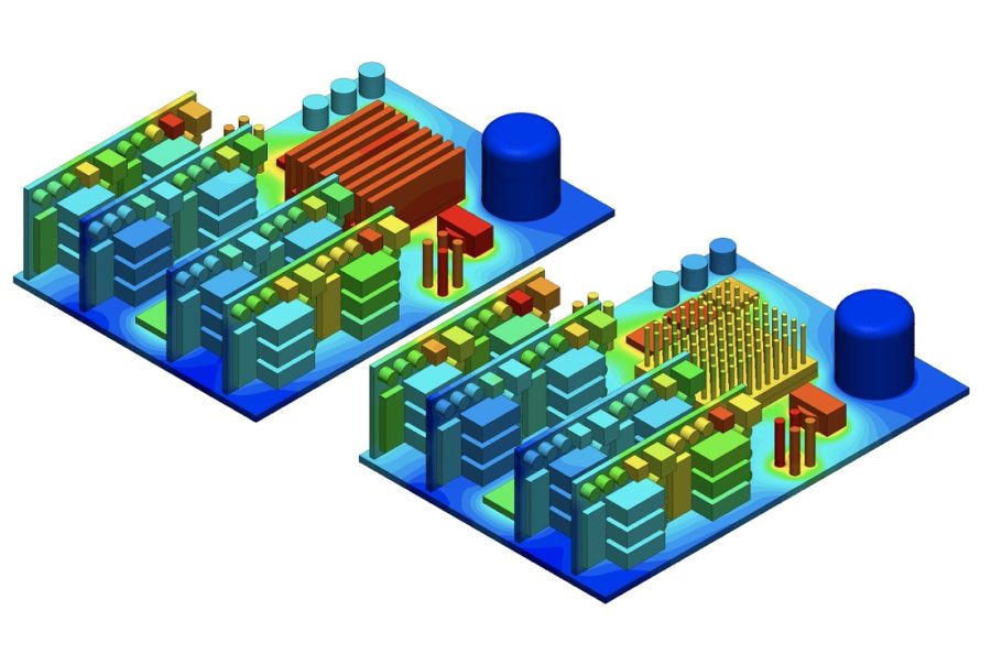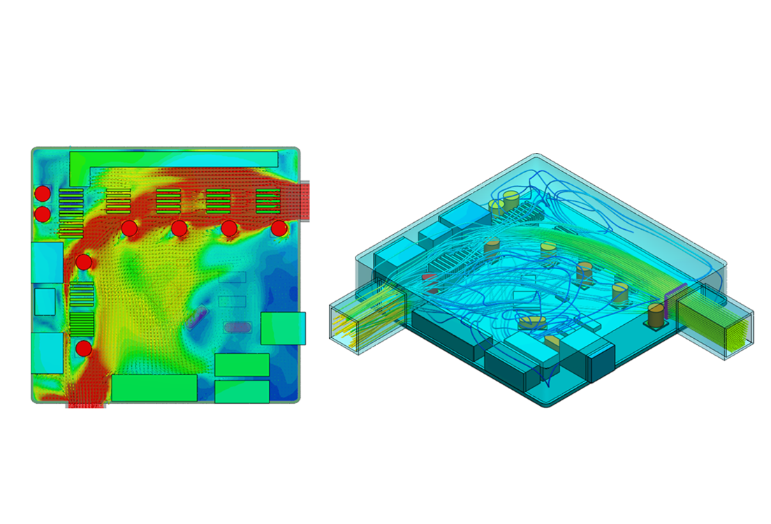
How to run a conjugate heat transfer (CHT) simulation

A CHT simulation answers the question a flow-only model cannot: how hot the components themselves get, not just the air moving past them. That is the number every thermal design decision hangs on, from heat sink sizing to whether a housing can be plastic.

This walks through the setup end to end, how to check the result against physical test, and what to watch for on lattice and TPMS models.

What a CHT simulation solves

CHT gives you component temperatures rather than fluid temperatures, without needing a heat transfer coefficient as an input.

A conduction-only thermal model requires an HTC at every wetted surface, which means supplying the answer to the hardest part of the problem. A flow-only model gives you insight into fluid cooling effectiveness but misses the resulting component temperatures, which matter most toward the center of components. CHT resolves both fields simultaneously and computes the coupling.

It covers conduction, forced convection, and natural convection in one model, additional to radiation where surface temperatures are high enough to matter. For the underlying theory, see the CHT analysis documentation.

When to use CHT, and when not to

Use CHT when you need solid temperatures, when conduction and convection compete, or when no correlation covers your local heat transfer coefficient.

Use CHT	Use something simpler
You need junction, component, or wall temperatures	You only need bulk fluid temperatures
Conduction and convection are both significant	One mode clearly dominates
Local HTC is unknown: recirculation, shrouded fins, dead corners	A published correlation or thermal resistance curve covers your case
Comparing variants where the flow field changes	First-pass power budget
Solid geometry is thermally significant	Geometry is simple enough to reduce to a resistance network

Setting up a CHT simulation

The setup follows the simulation tree: geometry, global settings, model, materials, boundary conditions, mesh, initial conditions, result control.

Step 1: Prepare the geometry

Upload the CAD and check that parts which should touch actually touch. Complex assemblies do not need simplification, because the cartesian meshing approach defeatures small geometrical details on its own.

Two geometry conditions are worth knowing about:

Gaps between parts that should be in contact are the ones that cost you. Heat will not transfer across a contact that is not there.
Overlaps and intersections are handled for you. The CHT solver warns and blocks the run so you can fix them; CHT (IBM) is not blocked by them and attributes the overlap to one of the parts.

If the model does not already contain the fluid region, create it with the flow volume extraction tools in the CAD Edit environment. An internal operation creates the volume inside a housing, an external operation creates a domain around the model. For an internal volume, a seed face touching the fluid is required, and boundary faces are only needed where the model has openings. The result is a solid CAD body you can assign a fluid material to.

Step 2: Global settings

Set time dependency, turbulence model, compressibility and radiation here.

Time dependency. Steady state answers what temperature something reaches given infinite time, which suits most thermal sizing. Transient is for duty cycles, thermal soak and warm-up.
Turbulence. k-omega SST is a sound default for forced convection. Laminar is reasonable for genuinely low-velocity natural convection.
Compressible. This decides whether buoyancy is treated in full or through the Boussinesq approximation. Toggle it on for air cooling where you want natural convection included, and switch pressure inputs to absolute (101325 Pa at sea level).
Radiation. Available in CHT and worth enabling once surface temperatures are high enough to matter.

Step 3: Model

Define the gravity vector under Model, referenced to the global coordinate system. It drives buoyancy, so a missing or wrongly oriented vector will give you a wrong natural convection result.

Step 4: Materials

Assign solids from the housing inward, and treat layered or wound components as anisotropic.

PCBs are alternating dielectric and copper layers, most commonly FR4, so conductivity is directional. In-plane runs high, often around 20 W/m·K, because heat spreads along continuous copper planes. Through-plane is usually below 1 W/m·K. Sum layer resistances in series for through-plane, combine in parallel for in-plane.
Transformers and motor windings behave the same way. An averaged conductivity underpredicts lateral spreading, which shows up as hot spots that are too sharp and too hot.

Step 5: Boundary conditions and heat sources

Most commonly you define flow at the inlet and let the outlet float, though this is application specific: exhaust and suction fans are defined at the outlet instead.

Inlet: flow rate or fixed velocity, plus incoming fluid temperature
Outlet: outlet boundary conditions for inner flow regions with forced flow. Natural convection inlet/outlet belongs on natural convection boundaries.
Heat loads: Power Source items under Advanced Concepts, applied to volumes in most cases, though bounding face heat loads are not uncommon

Specifying velocity at both inlet and outlet over-constrains the problem.

Use measured or datasheet power figures per component. Spreading a total system power evenly will put your hot spot in the wrong place.

If a fan or pump drives the flow, use its performance curve rather than a fixed velocity. The operating point moves as internal geometry changes, and a fixed velocity assumes away the interaction you are studying.

Step 6: Mesh

Check mesh quality before running. The platform warns in the event log when metrics fall outside the recommended range for your simulation type and mesh type, so there is no single number to aim at.

Three sizing modes are available:

Automatic: a single fineness level from 0 (coarse) to 10 (fine). This one can be driven by a parametric study, which makes a mesh sensitivity check straightforward
Manual: maximum and minimum edge lengths, with automatic refinement where geometry or physics warrants it
Custom: cells per direction plus refinement levels, each level halving cell size

Raise the resolution until the quantity you are reporting stops moving. How much movement is acceptable depends on the temperature range in play, so judge it against your own design margin rather than a fixed threshold.

Step 7: Initial conditions

Initialize fluids at the inlet temperature and solids at a sensible estimate of their final temperature. This mainly helps the run avoid diverging.

In a steady-state run the initial condition does not change the answer.

Step 8: Result control and convergence

Set result monitors before you start the run, because residuals alone are not the test. They can fall steadily while a hot spot is still climbing.

Inlet and outlet surfaces (mass flow, average temperature)
Every heat-generating body (volume average and maximum temperature)
Any surface you will report on

The run is converged when those quantities flatten and stay flat.

Check the energy balance too. Power in should match energy carried out by the fluid within a few percent. A mismatch means a leaking domain or a boundary condition that is not behaving as intended.

Validating against physical test

Compare against physical test at two ambient conditions rather than one. A single match can be coincidence; two points bracket the model across its operating range.

Pektron does this on bespoke automotive control units. They isolate the primary heat-generating chips in CAD, apply simplified geometry with a heat source, then run at 25°C and 85°C ambient to mirror their UKAS-accredited environmental chambers. Predictions track within 5°C of measured results.

That margin is what makes the model worth acting on. Pektron’s initial assumption was that the high-side drivers needed a heavy die-cast metal enclosure to act as a heat sink. The thermal model showed a lightweight aluminum pressing was enough.

Andrew Ashby

Mechanical Engineering Manager, Pektron

“By testing a few options in simulation up front, I could be confident that we didn’t need a full metal enclosure.”

With no test data to compare against, the fallbacks are the energy balance check from step 8, a mesh sensitivity study, and a Nusselt number check against a published correlation for a simplified version of your geometry.

Two worked examples

The two cases below sit at opposite ends of the CHT range: forced convection in air, and natural convection in liquid.

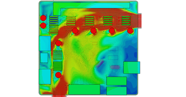
Forced convection: rugged edge computer

OnLogic used CHT to develop the Karbon 700, a rugged edge computer with thermal targets beyond anything they had attempted.

Deliberately modeled as a worst-case low-airflow installation
Multiple heat sources evaluated against chassis performance
3 to 5 mechanical design iterations run in parallel within one week
Each run finished inside 12 hours

Results landed within roughly 95% of measured product test performance. The design change that came out of it matched the thermal performance of a costlier alternative using less material, worth about $3 per system across thousands of units.

CHT simulation results showing airflow over heat sinks in an electronics enclosure

Post-processing results showing high flow over heat sinks at the inlet

Natural convection: immersion-cooled data center hardware

Submer evaluated five cooling designs for SmartPod, which submerges IT hardware in a dielectric liquid bath.

Both the CHT solver and the convective heat transfer solver used
Laminar throughout, on the grounds that natural convection in the bath never reached velocities justifying a turbulence model
Heat sink sizes and shapes reshaped around buoyancy-driven flow profiles rather than fan-driven ones
1,000 iterations per run, 1.5 to 2.5 hours on 32 cores
Earlier simulations duplicated as blueprints for later variants

Submer reports up to 95% lower cooling energy cost against traditional air cooling for their customers.

Insights relevant when dealing with lattice or TPMS models

Cartesian meshing handles lattice and TPMS geometry far more easily than a body-fitted approach, which is what makes this class of heat exchanger practical to simulate at all.

Siemens Energy designs additively manufactured heat exchangers as implicit geometry in nTop and runs CHT with the immersed boundary method in SimScale. Because SimScale reads the native implicit model directly rather than a faceted approximation, import drops from hours to seconds. On one heat exchanger the triangulated geometry reached roughly 6 GB and took several hours to generate and import.

What to plan for:

Mesh sizes of 50 to 150 million cells. Siemens Energy runs these on 192-core instances
Two competing objectives, evaluated in the same run: maximum heat transfer against minimum pressure drop
Parameters that move the result: TPMS cell type, cell size, wall thickness, surface roughness, and inlet and outlet design
Headless execution through nTop Automate and the SimScale API, which is what makes programmatic design loops practical at this cell count

Markus Lempke

Computational Designer, Siemens Energy

“Implicit modeling and direct simulations on implicit geometry is a real step change in speed and robustness of optimization workflows and necessary to unlock the real potential of additive manufacturing.”

cross-ING took the same route on an aluminum heat exchanger and a TPMS radiator, running incompressible flow first to check flow distribution and pressure drop, then CHT with immersed boundary methods for thermal performance. They varied lattice cell size across the volume to even out flow distribution while keeping the part printable.

Common CHT mistakes

Several of these produce output that looks reasonable, which is what makes them worth knowing.

Mistake	What you see
Gaps between parts that should be in contact	No heat transfer across the contact
Gravity undefined or wrongly oriented	Natural convection comes out wrong
Averaged conductivity on a PCB or winding	Hot spots too sharp and too hot
Residuals trusted over result monitors	Converged-looking run with a still-climbing hot spot
Total system power spread evenly across components	Hot spot in the wrong place
Velocity specified at both inlet and outlet	Over-constrained problem

Choosing CFD software for CHT

Four questions separate CHT CFD tools in practice, and raw solver speed is not one of them.

How long does a variant take end to end? Total time including CAD handling, meshing, queueing and post-processing. Solver time rarely dominates.

Can you run variants in parallel? Thermal design is comparative work. Running sequentially means exploring fewer designs regardless of single-run speed.

How much CAD preparation does it demand? Detailed assemblies should not need hours of simplification before they will mesh.

Is there anisotropic material support? Non-negotiable for PCB and winding work.

SimScale runs CHT in the browser with no hardware to provision, and runs variants in parallel rather than in a queue. Specifics on the thermal analysis page and pricing.

Frequently Asked Questions

What is a CHT simulation?

A simulation that solves heat conduction through solids and heat carried by moving fluid at the same time, in one model, so heat transfer at the solid-fluid boundary is calculated rather than assumed.

How do I set up a CHT model?

Follow the simulation tree: prepare the geometry, set global settings including turbulence and compressibility, define gravity under Model, assign materials, apply boundary conditions and power sources, mesh, set initial conditions, then add result control items.

Why is my CHT simulation not converging?

Common causes are velocity specified at both inlet and outlet, a missing or wrongly oriented gravity vector, and initial conditions far from the expected solution. Check the energy balance as a diagnostic: power in should match energy carried out by the fluid within a few percent.

How long does a CHT simulation take?

Hours rather than minutes, scaling with mesh size. Submer’s immersion cases ran 1.5 to 2.5 hours on 32 cores; OnLogic’s electronics runs finished inside 12 hours.

What mesh do I need for CHT?

Start at an automatic fineness level and raise it until the quantity you are reporting stops moving. Check mesh quality before running; the platform warns in the event log when metrics fall outside the recommended range for your simulation and mesh type.

What turbulence model should I use for CHT?

k-omega SST for forced convection. Laminar for genuinely low-velocity natural convection.

When should I toggle compressibility on?

For air cooling where you want natural convection included. The setting decides whether buoyancy is treated in full or through the Boussinesq approximation, and it switches pressure inputs to absolute.

Can I run CHT on a TPMS or lattice heat exchanger?

Yes. Cartesian meshing handles that geometry far more easily than a body-fitted approach, and works directly on implicit geometry. Expect 50 to 150 million cells.

How do I model a PCB in a CHT simulation?

As an anisotropic solid. In-plane conductivity is high, often around 20 W/m·K, through-plane usually below 1 W/m·K. Sum layer resistances in series for through-plane, combine in parallel for in-plane.