Validation Case: Laminar Pipe Flow with Multi-purpose Solver

The aim of this test case is to validate the following parameters of incompressible steady-state laminar fluid flow through a pipe with the Multi-purpose solver:

• Velocity
• Pressure drop

The simulation results of SimScale were compared to the analytical results obtained using the Hagen-Poiseuille equations\(^1\).

Geometry

A straight cylindrical pipe was chosen as the flow domain (see Figure 1). Faces A, B, and C represent the inlet, wall, and outlet, respectively.

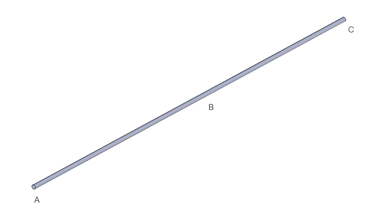
Dimension	Length	Diameter
Value \([m]\)	2	0.01

Analysis Type and Mesh

Analysis Type: Multi-purpose steady-state analysis.

Turbulence Model: Laminar flow

Mesh and Element Types:

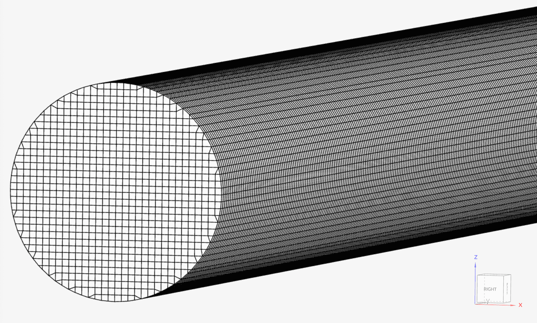
Three structured, body-fitted Cartesian meshes are generated on the SimScale for this validation case (see Figure 2). The meshes are refined with a growth rate of around 8. Later, these meshes are used to verify the mesh independence of the results.

With the mesh strategy used, all 3 resulting meshes are uniform, each having a constant edge length over the entire volume. The global cell size and refinement sizes are defined as follows:

Mesh Name	Edge Length \([m]\)	Number of cells
Coarse Mesh	1.25E-03	83200
Moderate Mesh	6.25E-04	665830
Fine Mesh	3.125E-04	5222400

Simulation Setup

Fluid:

• Water:
  • \((\nu)\) Kinematic viscosity = 10^-6 \(\frac{m^2}{s}\)
  • \((\rho)\) Density: 1 \(\frac{kg}{m^3}\)

Boundary Conditions:

Face	Boundary type	Value
Inlet (A)	Velocity inlet	0.1 \(m/s\) in the y-direction
Outlet (C)	Pressure outlet	Fixed value of 0 \(Pa\)
Wall (B)	Wall	No-slip

One of the parameters of interest, which is the topic of this validation case, is the pressure drop through the pipe. Above all, the Hagen–Poiseuille equation considers the flow at the inlet to be fully developed. There are two common CFD methods to generate a fully developed flow:

• Method 1: Firstly, approximate the laminar entry length. Then extend the pipe inlet by adding the entry length. The flow becomes fully developed after the entry length is achieved. As a result, this measure ensures the correct velocity profile at the pressure measurement points.
• Method 2: At the inlet, define a parabolic velocity profile, which matches with the Hagen-Poiseuille parabolic velocity equation.

As Table 3 above indicates, in this validation case, the first method is employed. A tube with a diameter of 0.01 meters and a length of 2 meters is used, with the objective of allowing the flow to develop and only using the portion of the tube that has a developed profile for validation purposes.

Analytical Solution

The analytical solution gives us the following equations for maximum axial velocity, pressure drop, and developed radial velocity profile:

$$u_{y \ max} = 2u_{y \ avg}$$

$$\Delta P = \frac{128}{\pi} \frac{\mu L}{D^4} Q $$

$$u_y = -\frac{1}{4\mu} \frac{\partial p}{\partial y}(R^2 – r^2)$$

where,

• \( u_{y\ avg} \): Average inlet velocity, equal to 0.1 \([m/s]\)
• \( u_{y\ max} \): Maximum velocity that occurs at the centerline \([m/s]\)
• \( u_{y} \): Velocity along the axis \([m/s]\)
• \(r\): Radial distance from the centerline \([m]\)
• \(R\): Radius of the circular pipe \([m]\)
• \(\Delta P\): Pressure loss \([Pa]\)
• \(\mu\): Dynamic viscosity \([kg/(m\cdot s)]\)
• \(L\): Length of circular pipe \([m]\)
• \(D\): Diameter of circular pipe \([m]\)
• \(Q\): Volumetric flow rate \([m^3/s]\)
• \(\frac{\partial p}{\partial y}\): Pressure gradient along the pipe \([Pa/m]\)

Result Comparison

Given that a uniform velocity definition is used at the inlet, before further processing the results, it is important to understand how much length the velocity profile takes to develop. In the fine mesh results, the velocity in the y-direction is plotted over a line from the center of the inlet to the center of the outlet:

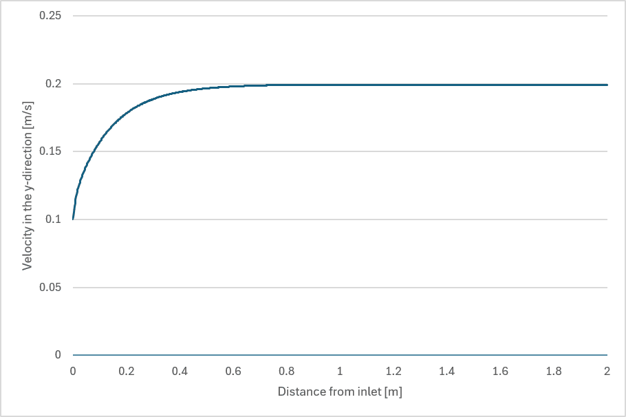
At around 0.8 meters from the inlet (80 diameters), the inlet velocity stabilizes. As such, only the results from 1 meter from the inlet up to the outlet (1 meter of length in total) will be further analyzed below.

A mesh sensitivity was conducted, aiming to compare the maximum velocities in the y-direction observed at the outlet. As discussed in the previous section, the analytical result is twice the average velocity; therefore, for this case, the maximum expected velocity is 0.2 \(m/s\):

Mesh Name	Number of Cells	Analytical Maximum Velocity in y \([m/s]\)	Maximum Velocity in y \([m/s]\)	Error (%)
Coarse Mesh	83200	0.2	0.188	-6
Moderate Mesh	665830	0.2	0.198	-1
Fine Mesh	5222400	0.2	0.199	-0.5

The maximum velocities change by less than 1% between the moderate and fine meshes, and both of them are within 1% of the analytical solution, indicating mesh convergence.

Focusing now on the fine mesh results, we want to compare the pressure drop experienced by the flow in the second half of the tube (from 1 to 2 meters away from the inlet). The analytical delta pressure considering a 1-meter length tube is 0.32 \(Pa\).

Table 5 contains a compilation of average static pressure values at different distances from the inlet:

Distance from the Inlet \([m]\)	Analytical Static Pressure \([Pa]\)	Static Pressure (Fine Mesh) \([Pa]\)	Error (%)
1	0.03200	0.03216	0.51
1.1	0.02880	0.02894	0.51
1.2	0.02560	0.02573	0.50
1.3	0.02240	0.02251	0.49
1.4	0.01920	0.01929	0.48
1.5	0.01600	0.01608	0.49
1.6	0.01280	0.01286	0.49
1.7	0.00960	0.00964	0.46
1.8	0.00640	0.00642	0.41
1.9	0.00320	0.00321	0.31
2.0	0.00000	0.00000	0.00

The simulation results are consistent with the analytical solution throughout the analyzed pipe length.

Lastly, the radial velocity profile is analyzed, with a comparison between the simulation results at the outlet section to the analytical solution. Note that the simulation results consist of cell data (i.e. not interpolated):

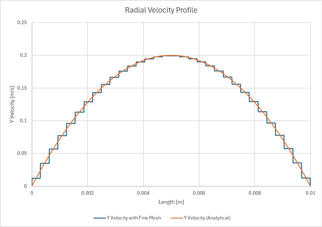
Overall, the developed velocity profile with the fine mesh shows exceptional correlation with the analytical results over the entire diameter.

Last updated: July 30th, 2025