Documentation
The aim of this validation is to compare the simulation results performed in SimScale using the transient compressible flow feature in its proprietary solver, Multi-purpose, with the analytical results obtained using the Compressible Flow Equations\(^{1,2,3}\).
The objective is to test the Multi-purpose solver’s ability to compute supersonic inviscid flows and, in particular, to capture normal shock waves at exact locations inside a converging-diverging (CD) nozzle.
The CD nozzle geometry used for validation purposes is as follows:
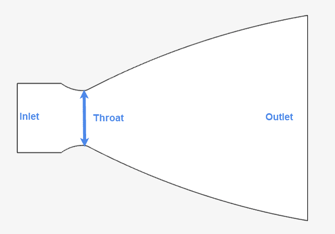
The dimensions are tabulated below:
| Dimension | Value \([m]\) |
| Inlet | 0.8 |
| Outlet | 2.372 |
| Inlet-outlet distance | 3.362 |
| Throat | 0.6336 |
| Inlet-throat distance | 0.777 |
The geometry has a tiny thickness to represent a two-dimensional flow. This means that the cross-section is a rectangle instead of a circle. This helps to save on computational expenses while still maintaining the physics and the numerical accuracy required.
Analysis Type: Transient, Multi-purpose with k-epsilon and Compressible model
Mesh and Element Types:
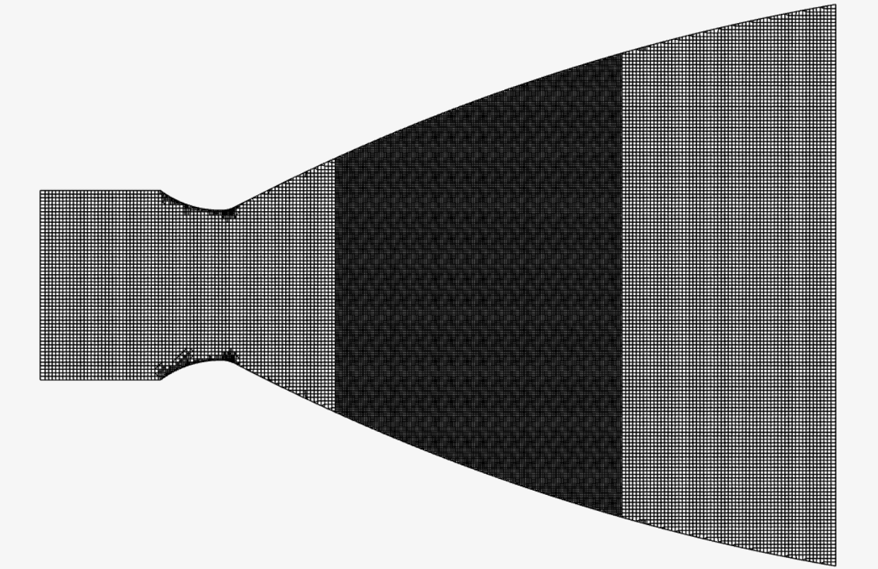
The mesh was created with SimScale’s Multi-purpose mesh type, which is a body-fitted structured mesh. An automatic sizing definition was defined with an additional region refinement near the normal shock location.
| Mesh Type | Fineness | Target Cell Size (refinement) \(m\) | Number of cells | Element Type |
| Automatic with region refinement | 2 | 0.01 | 163959 | 3D Hexahedral |
The resulting mesh is as observed below:
Fluid:
Figure 4 shows the schematic of the boundary conditions applied:
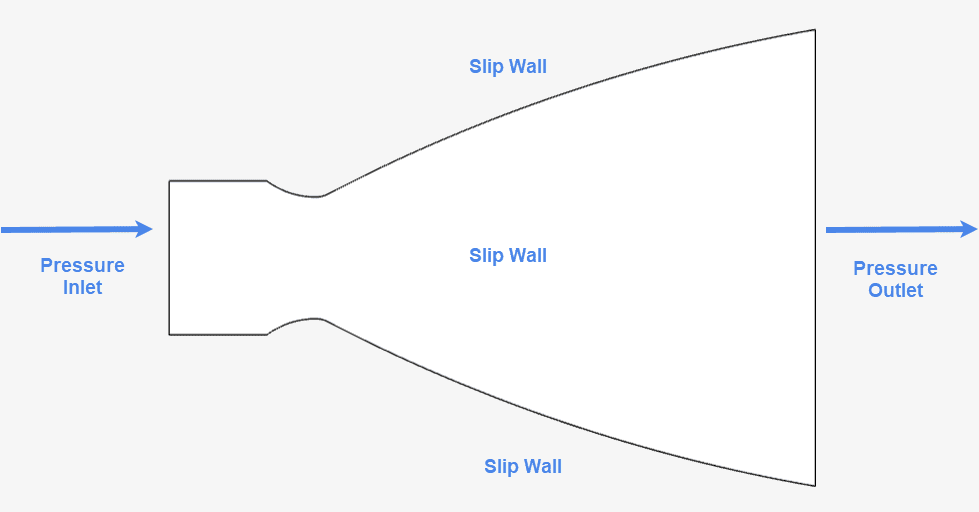
| Boundary Condition | Value |
| Pressure inlet \([Pa]\) | 699325 (Absolute total pressure with 19.85 \(°C\) total temperature) |
| Pressure outlet \([Pa]\) | 360201.02 (Fixed absolute static pressure) |
| Slip wall (adiabatic) | Remaining faces |
Using the continuity equation and isentropic relations, for every geometry and one selected fluid with the specific heat ratio \((\gamma)\), a unique correlation between the cross section area \((A)\), throat area \((A^*)\), and Mach number \((M)\) measured upstream from that cross section is defined as follows\(^{1,2,3}\):
$$ \frac{A}{A^*} = \frac{1}{M} \left[\frac{2}{\gamma + 1} \left(1+ \frac{\gamma\ -\ 1}{2}M^2 \right) \right]^ \frac{\gamma + 1}{2(\gamma\ -\ 1)} \tag{1}$$
Considering the properties of the geometry shown in Figure 1, the Area-Mach number relation in Equation 1 is used to calculate the exact Mach number in every cross section of the nozzle.
For this validation purpose, we will calculate the Mach number at the shock location of 1.5 \(m\). The supersonic Mach number for this location is obtained to be 2.38254.
The next step is to calculate the correct ratio of the stagnation pressure at the inlet to static pressure at the outlet, which results in a normal shock within the diverging part of the nozzle at \(x\) = 1.5 \(m\).
Did you know?
Due to the nature of the Area-Mach number relation, for each cross-section area, two solutions for the Mach number are obtained – one in the supersonic and one in the subsonic regime.
Using the theory of compressible flow equations \(^{1,2,3}\), it was found that for the normal shock to appear at 1.5 \(m\), the ratio of outlet static pressure to inlet stagnation pressure should be 0.51507.
Accordingly, the values were chosen for the inlet and outlet pressure discussed in Table 2 above.
The result output from the SimScale simulation is compared with the analytical results\(^{1,2,3}\).
The normal shock is very well-defined within the diverging part of the nozzle. This can be studied in Figure 4 and Animation 1.
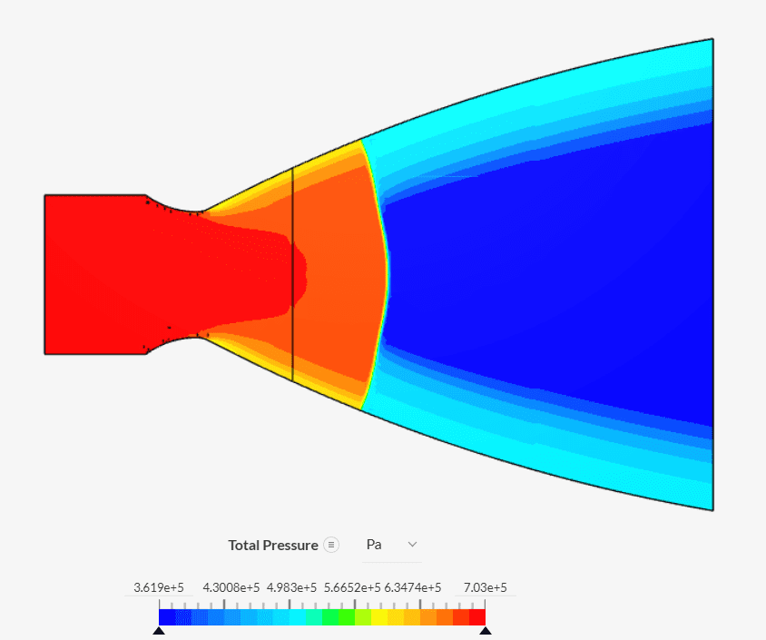
The shock is produced exactly at \(x\) = 1.5 \(m\). The Mach number at this location is observed to be 2.385. These quantities were calculated using the tools in SimScale’s integrated online post-processor.
The above animation shows the changing location of the normal shock in a converging-diverging nozzle as time progresses, in a transient simulation, until it settles at \(x\) = 1.5 \(m\).
In conclusion, the normal shock location and the Mach number obtained using SimScale’s Multi-purpose solver exactly match those calculated using the analytical equations.
References
Note
If you still encounter problems validating your simulation, then please post the issue on our forum or contact us.
Last updated: June 30th, 2025
We appreciate and value your feedback.
Sign up for SimScale
and start simulating now