Documentation
With the increase in the number of high-rise buildings being constructed all around the world, proper planning of the close vicinity for comfort and safety becomes important. Computational fluid dynamics (CFD) is an ideal solution for assessing these comfort and safety levels for pedestrian wind comfort (PWC) even before the buildings are erected, and it also helps enable faster design iterations. Pedestrian-level (micro-climate) condition is one of the first microclimatic issues to be considered in modern city planning and building design \(^1\).
Wind analysis results using CFD simulation are now seen as reliable sources of quantitative and qualitative data, and they are frequently used to make important design decisions. However, to have full confidence in those decisions, extensive verification and validation of the CFD results are necessary. For this, we will validate the CFD results against the experimental results provided by the Architectural Institute of Japan (AIJ), using AIJ Case D.
The Architectural Institute of Japan (AIJ) is a Japanese professional organization for architects, building designers, and engineers. It was founded in 1886 and has gathered over 38,000 members since. It publishes several journals, technical standards for architectural design and construction, and research committee studies.
The wind analysis test case for this validation was taken from the “Guidebook for Practical Applications of CFD to Pedestrian Wind Environment around Buildings”\(^2\), published by AIJ in 2008, which sets the standards for cross-comparison between the results of CFD predictions, wind tunnel tests, and field measurements, and helps validate the accuracy of CFD codes for pedestrian wind comfort assessments.
The purpose of this project is to use experimental results from the Architectural Institute of Japan\(^3\) to validate CFD results gained from SimScale using the Lattice-Boltzmann Method (LBM) provided by Numeric Systems GmbH. The case being validated is Case-D, which consists of a single high-rise building of 100 \(m\) height, surrounded by blocks of simplified buildings. The Wind tunnel experiments were conducted at a scale of 1/400 on the model at the Niigata Institute of Technology and the inflow velocity at the central building height was 6.61 \(m/s \).
Moreover, the measurements were performed for 3 different wind directions: 0°, 22.5°, and 45°.
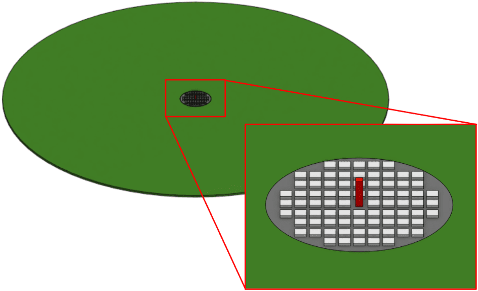
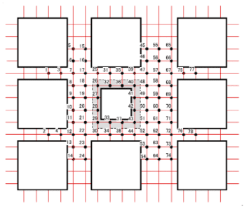
The CAD geometry was modeled based on the geometry data and specification that is available in the AIJ Case D datasheet \(^3\). The figure below shows the CAD model uploaded into SimScale with the main building highlighted in red, and an orange box representing the location of the measurement points which are shown in Figure 2.
For this simulation, we used SimScale’s LBM solver, which is a different approach to traditional Finite Volume Methods. This solver is an implementation of Pacefish®, provided by Numeric Systems GmbH\(^4\), and has many advantages over the traditional approach, but the most relevant in this case are geometry robustness and solver speed. Since the solver runs on GPU architecture and scales very well, we can solve transient simulations on very large meshes in a fraction of the time it would take traditional solvers to solve in steady-state.
A summary of the simulation setup is as follows:
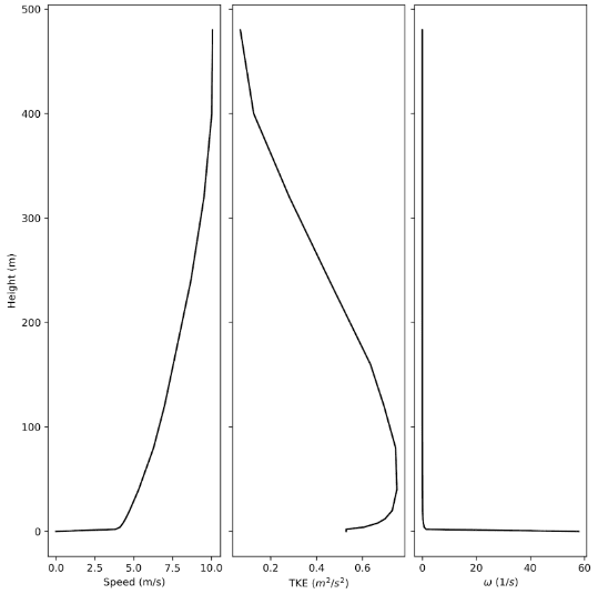
Regarding the ABL wind profile, a power law approximation was applied, as is the default for the SimScale Pedestrian Wind Comfort (PWC) approach. The figure below illustrates the log-law ABL profiles for velocity and turbulent quantities generated by SimScale.
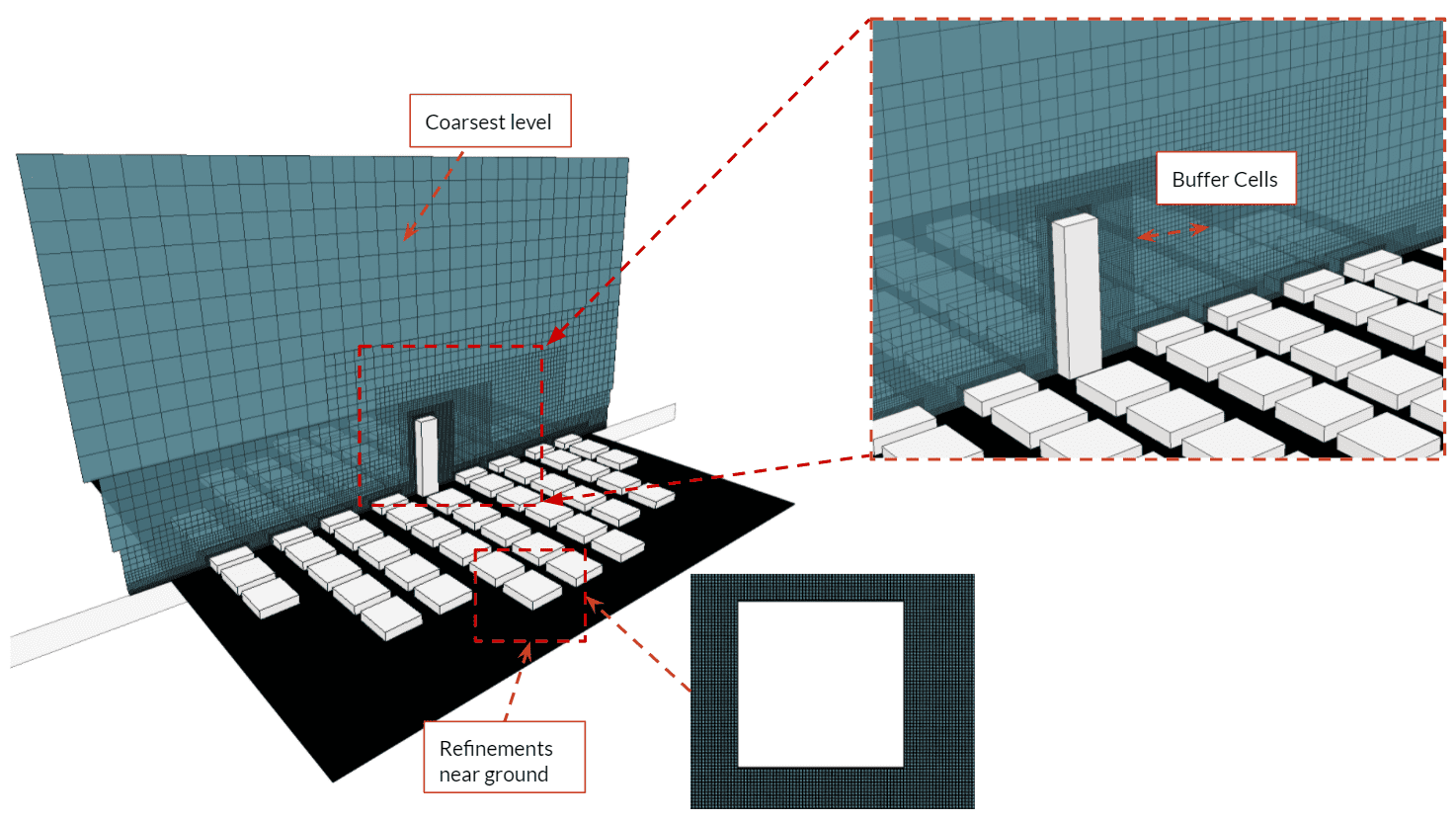
For an incompressible LBM analysis, the meshing is based on the lattice Boltzmann method (LBM) and is quite different from the finite-volume-based fluid dynamics analysis types in SimScale. Here a cartesian background mesh is generated, which is composed only of cube elements that are not necessarily aligned with the geometry of the buildings or the terrain.
To take into account the exact geometry, there exists a sub-grid model that accounts for the interfaces between the geometry and the fluid domains.
Turbulence Model
As mentioned before, the turbulence model K-omega SST DDES, which uses the highly regarded LES turbulence model in the far-field but uses the equally well-regarded wall model from the K-omega SST model, has proved itself particularly in the Aerospace Industry. The transition between the two models happens in the log-law region in the boundary layer. This means that we improve turbulence prediction by using LES, but also reduce its inherent cost by adding a robust wall model, reducing the mesh requirement at the wall.
Mesh information:
Mesh Convergence Study:
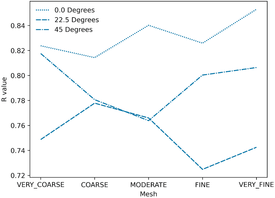
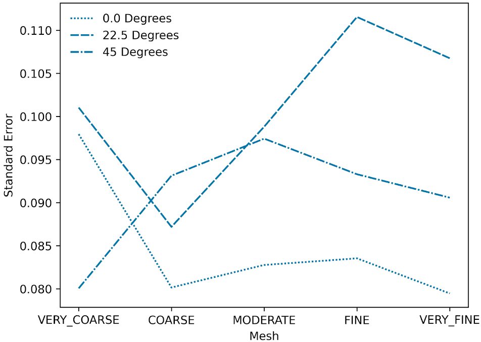
A mesh convergence study is conducted to eliminate the dependency of the results on the mesh size. This is illustrated in Figures 5 & 6 using the R-squared correlation coefficient and standard error between the velocity results obtained by SimScale and the experimental results from the wind tunnel.
Based on these results, the “fine” mesh was determined to be the point where the simulation has reached mesh-size independence, as the standard error has started to flatline and there is a sufficient balance between accuracy and computational efficiency.
The results obtained from the simulation are validated with the wind-tunnel experimental data, which are split into two experiments \(^3\) :
The results from the simulation were averaged over the latter 20% of the simulation time to exclude results that are distorted by the time it takes for the simulation to stabilize.
To set the basis for the comparison, the velocity results that were obtained at the measurement points (“validation points” in the simulation) were normalized by the inflow velocity of the wind tunnel experiment at the reference height of the center building. Which was 6.65 \(m/s\) at 100 \(m\) height.
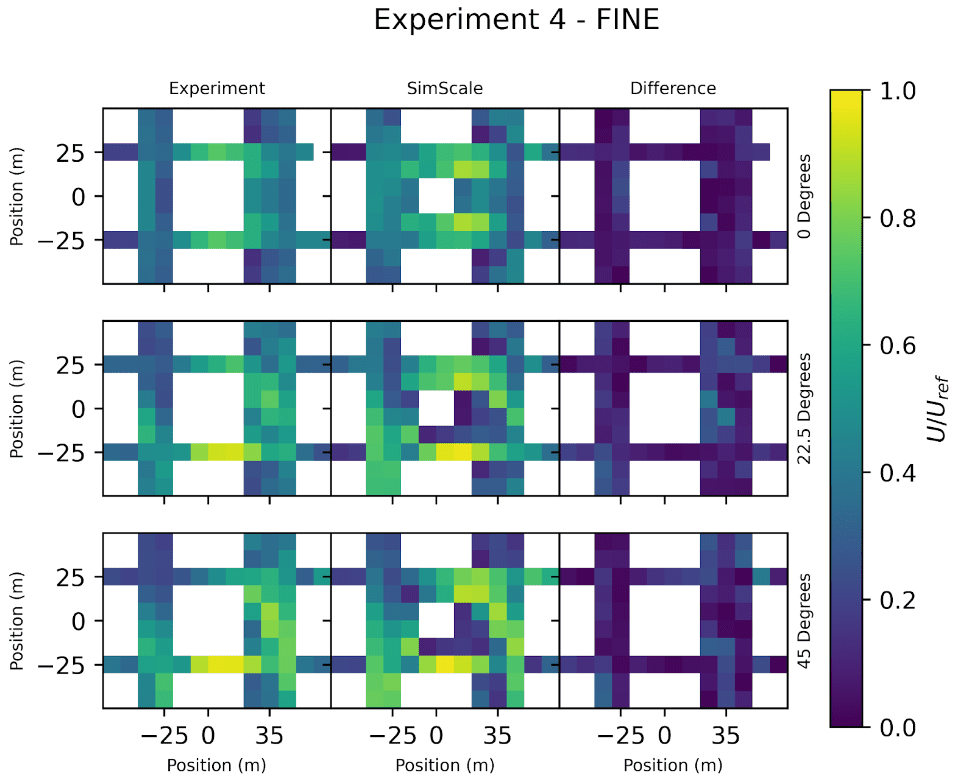
The results for the three analyzed wind directions are presented below in Figures 7 and 8 using several plots:
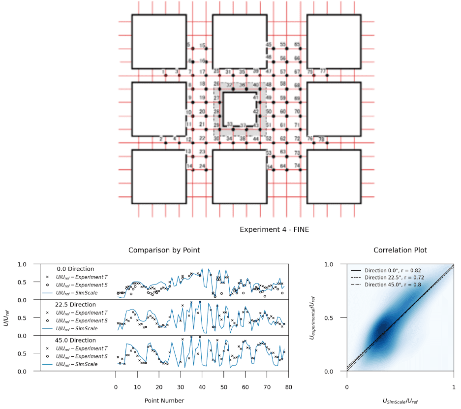
Looking at the results above, one can see that Pearson correlation coefficients of 0.82 (0° wind), 0.72 (22.5° wind), and 0.80 (45° wind) were obtained. Compared to the other mesh refinement levels, these represent the best overall agreement at a reasonably balanced computational cost.
Moreover, in the velocity comparison plots (7-8), one can directly inspect the approximation behavior of SimScale to the experimental results for the respective wind directions, and understand where it fits the data best, and where it deviates.
For the 0° wind condition, the main deviations are in points ~15-24, which represent the wake of the middle left (windward) building. There is also a small overprediction in the velocity jets around the central building (points 46-48 and 51-53). The off-direction flows (22.5° and 45°) exhibit very similar results to one another, with an overprediction in wind velocity in the leading probes (points ~5-10 and ~15-20) and an underprediction in the rearmost (leeward) probes (points ~65-75).
Overall a great qualitative and good quantitative agreement exists between experimental and SimScale-obtained CFD results. Results match best for points in the freestream (in streets and roads not affected by building wind shading) where there exists more of these points for lower angles of attack. For higher angles of attack, most points will be in building wind shade (the wake region), however, even here we show a good agreement with the wind tunnel experiment with R-values north of 0.7, thanks to the hybrid model.
The purpose of this study was to validate the LBM method provided by Numeric Systems GmbH against the wind-tunnel experimental results of AIJ Case D. The results had shown good correlation to the wind tunnel data provided, where correlation coefficients of 0.82, 0.72, and 0.80 were obtained for the 0°, 22.5°, and 45° wind directions, respectively. Moreover, by inspecting the approximative trend of the SimScale results, one can clearly visualize that it follows the pattern of the experimental data.
In general, both wind tunnel testing and CFD methods have their pros and cons and one cannot replace the other, especially when one understands that each is a different type of simulation that is suitable for different stages of a project and the type of information that you want to obtain from that particular study.
Typically, wind tunnel testing is mostly done for compliance testing and it is well known that it takes quite some time and great expense to set up the test and process the results. All these factors make it quite difficult or infeasible to integrate it into an early iterative design process. Engineers and designers derive the most value from CFD analysis because it allows them to obtain such a vital amount of information early on in the design process, with confidence that it will corroborate to wind tunnel studies when validated at the later stages.
Lastly, In terms of turnaround time, this validation quality mesh, consisting of 48.2 million cells, took just ~90 minutes to solve, with a resolution of 0.38 (m), and cost around 6 GPU hours. In comparison to wind tunnel modeling, this is a big cost and speed advantage. This also compares quite favorably against traditional finite volume CFD methods, which can take upwards of days of solve time for such a demanding mesh and turbulence model. The numerical robustness of the Lattice-Boltzmann solver also makes a huge efficiency difference, as there were no iterations to obtain numerical stability from the mesh, setup, and geometry quality, where experienced analysts will know this is where they traditionally spend the most amount of labor time.
References
Last updated: July 17th, 2023
We appreciate and value your feedback.
Sign up for SimScale
and start simulating now