Tutorial: Electrostatics Simulation on a High Voltage Power Cable

This tutorial showcases how to use SimScale to run an electrostatics simulation on a High Voltage Power Cable in order to evaluate the electric field magnitude and the capacitance matrix.

Overview

This tutorial teaches how to:

• Set up and run an electrostatics simulation;
• Assign multiple materials and other properties to the simulation;
• Mesh with the automatic standard meshing algorithm.

We are following the typical SimScale workflow:

1. Prepare the CAD model for the simulation;
2. Set up the simulation;
3. Create the mesh;
4. Run the simulation and analyze the results.

1. Prepare the CAD Model and Select the Analysis Type

To begin, click on the button below. It will copy the tutorial project containing the geometry into your Workbench.

The following picture demonstrates what is visible after importing the tutorial project.

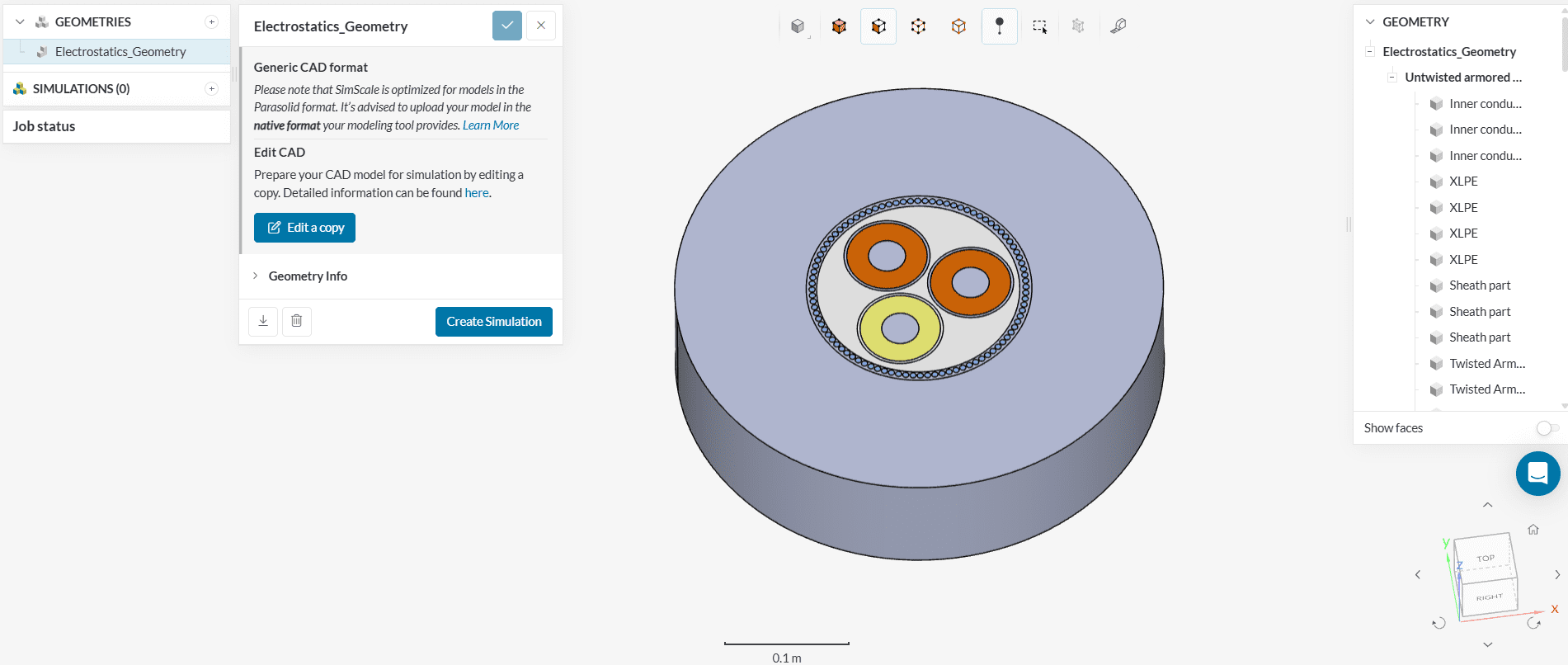
The geometry consists of an actual Power Cable assembly. It consists of multiple parts, as can be observed in the scene tree.

1.1 Geometry Preparation

The geometry contains multiple solid parts and is already ready for an electrostatic simulation.

1.2 Create the Simulation

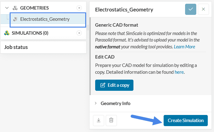
Click on the geometry ‘Electrostatics_Geometry’ and hit the ‘Create Simulation’ button. You can rename it if you’d like.

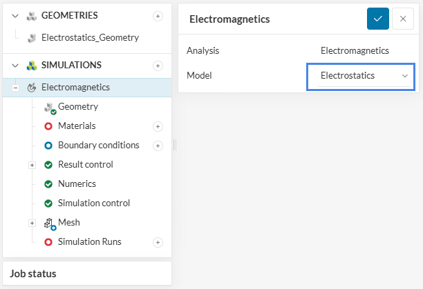
This will open the simulation type selection widget:

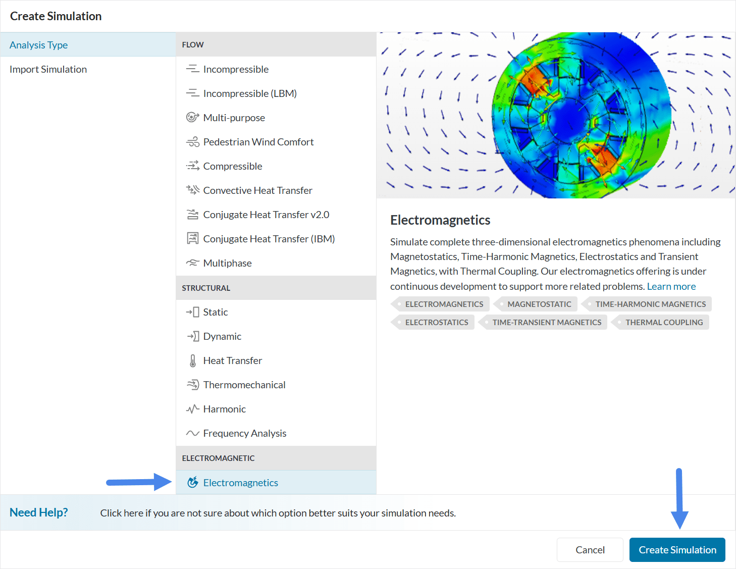
Choose ‘Electromagnetics‘ as the analysis type and ‘Create Simulation’. Since we are dealing with stationary electric fields and charges, this tutorial will be solved under the Electrostatics model.

At this point, the simulation tree will be visible on the left-hand side panel.

2. Pre-Processing: Setting up the Simulation

2.1 Define Materials

Material definition becomes very easy in an Electrostatics simulation such as this one since the only variable is the Relative electric permittivity.

First, click on the ‘+ button’ next to Materials. In doing so, the SimScale fluid material library opens, as shown in the figure below:

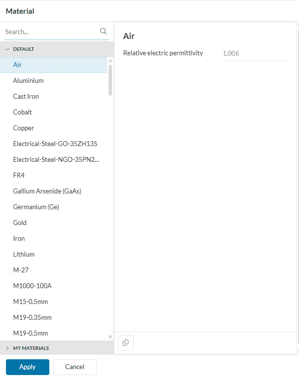
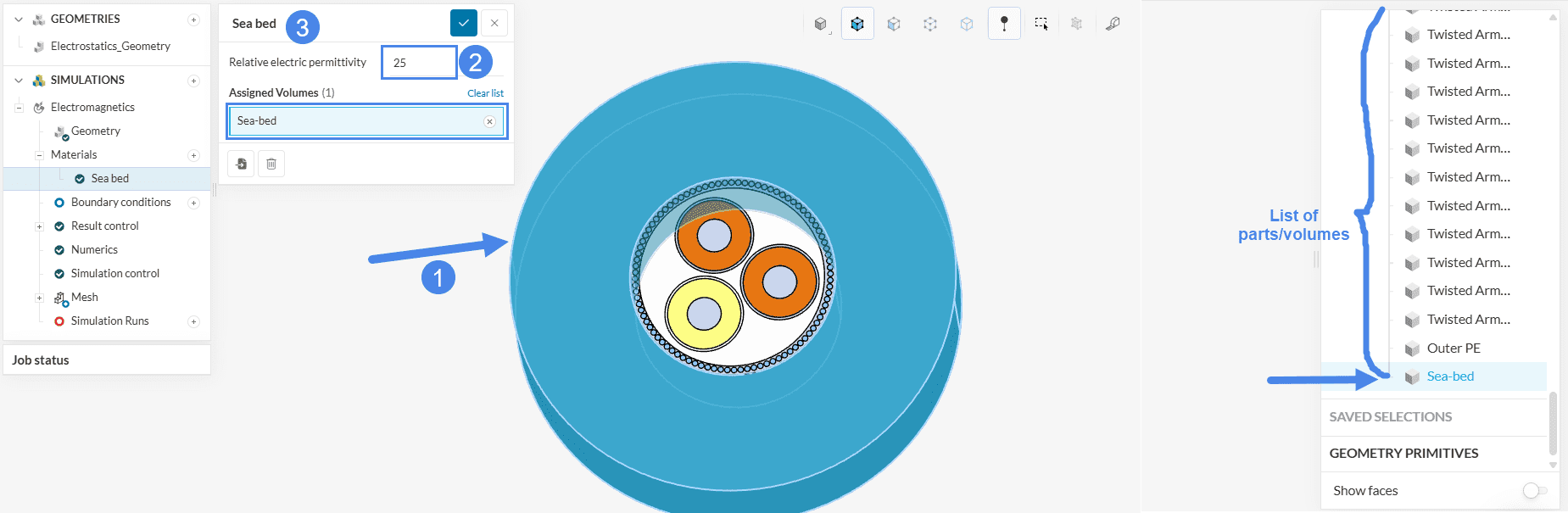
Select ‘Air‘ and click ‘Apply’. Assign the outer ‘Sea-bed’ volume to this material. This assignment can also be done from the list of parts on the right. Change Relative electric permittivity to ’25’ and rename the material to ‘Sea bed’. Click ‘Save’.

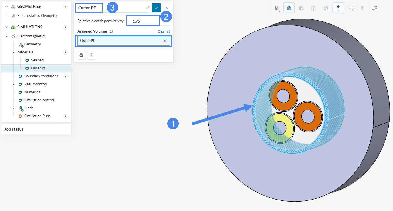
Repeat the same procedure for the ‘Outer PE’ volume and assign it a permittivity of ‘1.75’.

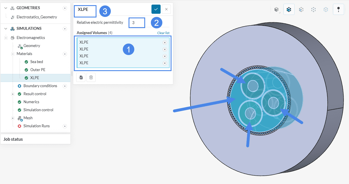
Repeat the same procedure for the 4 ‘XLPE’ volumes and assign them a permittivity of ‘3’.

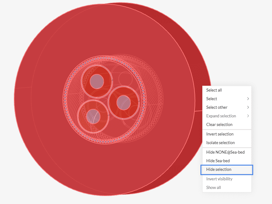
For the remaining material assignments we will hide the outer parts to view the ones inside. Select (left-click), right-click, and hide the volumes to which you already assigned a material.

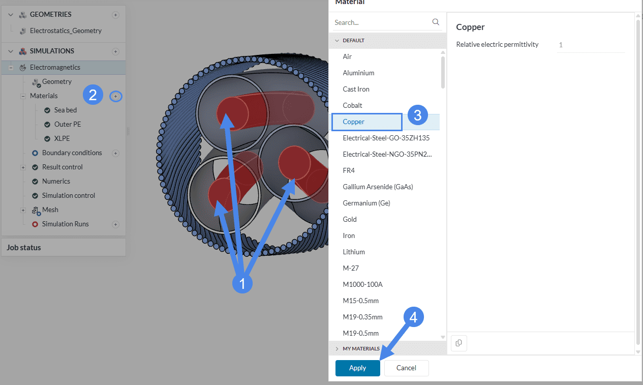
Now select the 3 ‘Inner conductors’ volumes and assign ‘Copper’ as their material directly from the material library.

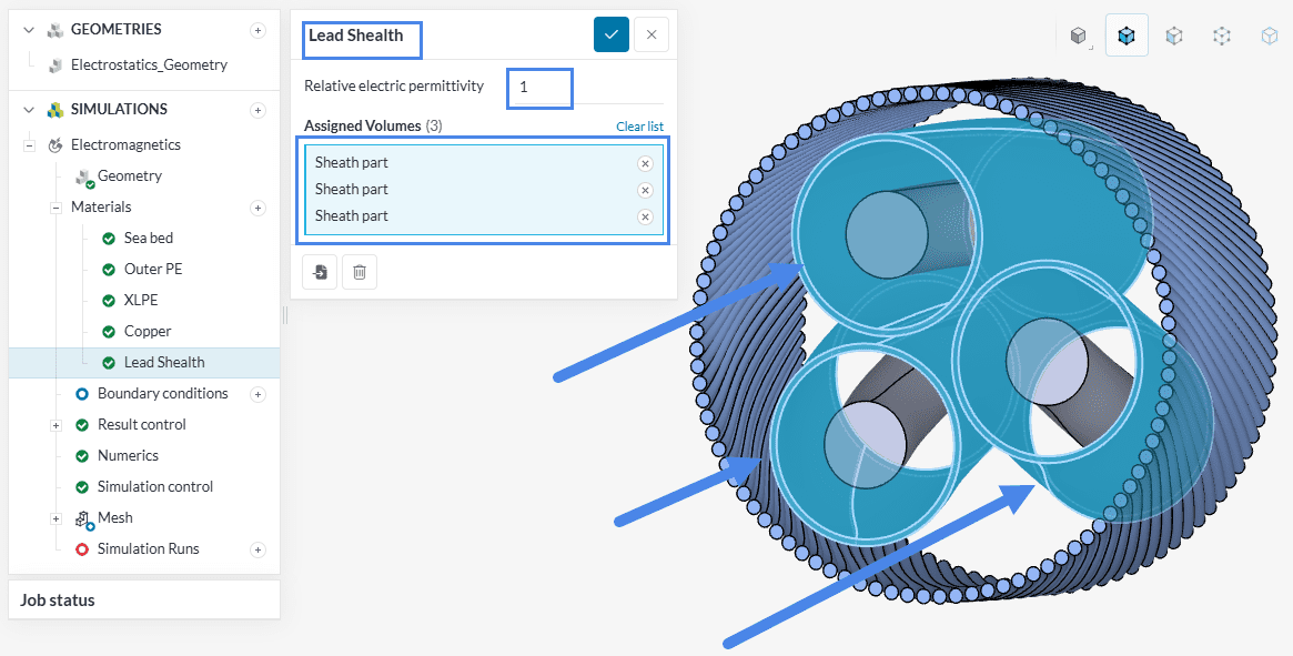
Repeat the procedure for the 3 ‘Sheath part’ volumes and rename it to ‘Lead Sheath‘.

Select and hide the copper conductors and the lead sheath volumes as done before to have only the twisted armor cables in view.

Add a ‘Stainless Steel’ material from the library.

Right-click on the Workbench and select ‘Assign all’.

Right-click on the Workbench again and select ‘Show all’ to display all volumes.

2.2 Assign the Boundary Conditions

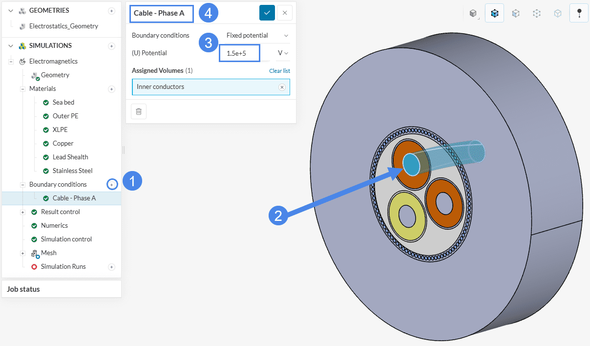
First, we shall set the voltage for each of the three High Voltage Power Cables.

First, click on the ‘+ button’ next to Boundary Conditions and select ‘Fixed potential’ boundary condition. Set the (U) Potential to ‘1.5e+5’ \(V\) and rename the boundary condition as ‘Cable – Phase A’.

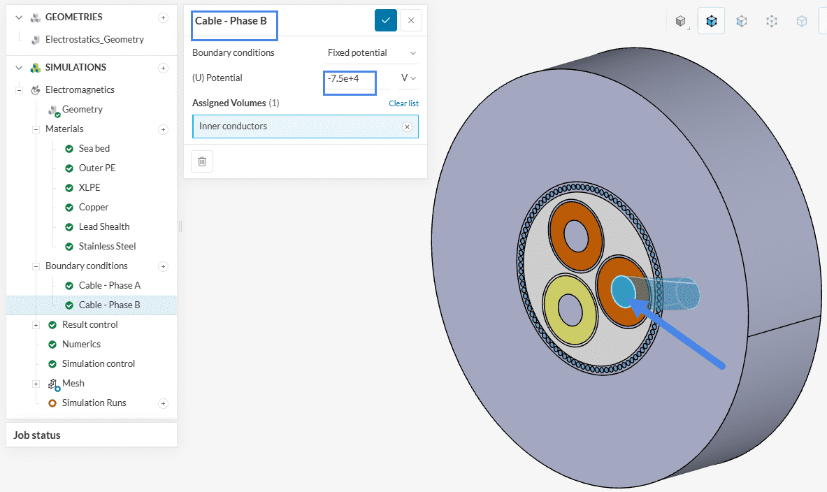
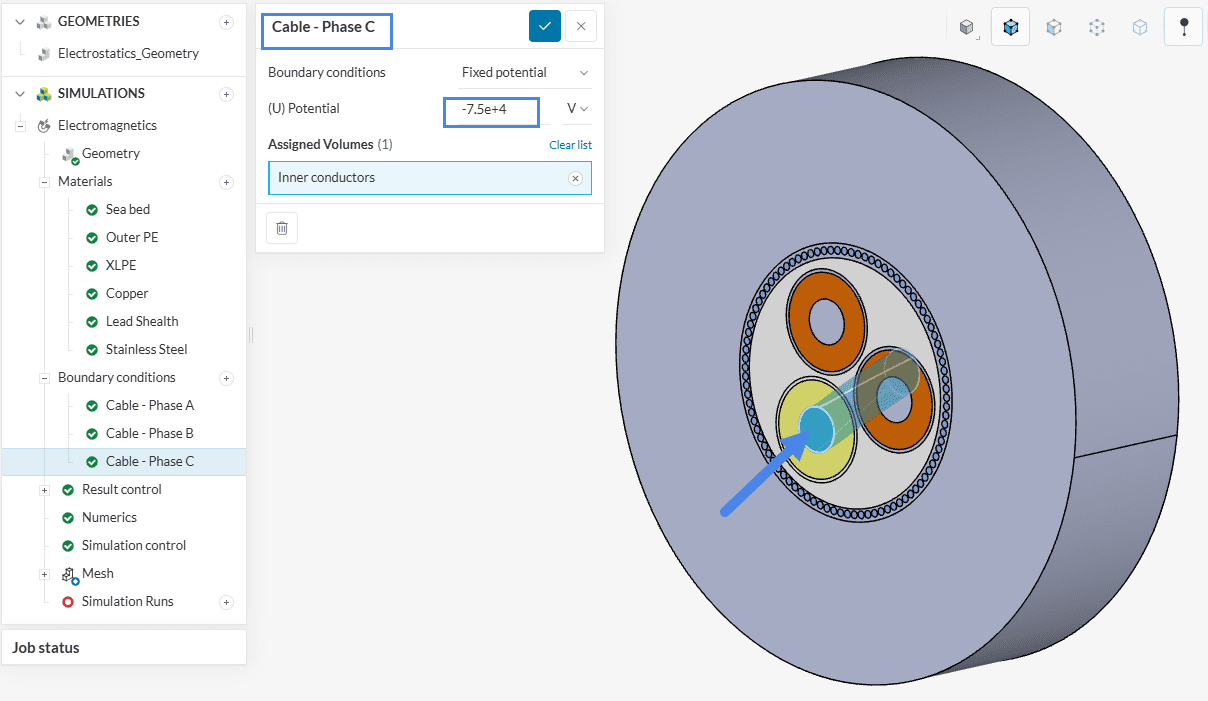
Repeat this process for the other two conductors and set their individual potential to ‘-7.5e+4’ \(V\) and name them ‘Cable – Phase B’ and ‘Cable – Phase C’.

Select and hide the Sea bed volume. To add a Ground, add another Fixed potential boundary condition with a potential of ‘0’, rename it as ‘Grounded‘ and assign it to the two outer faces of the Outer PE volume as follows:

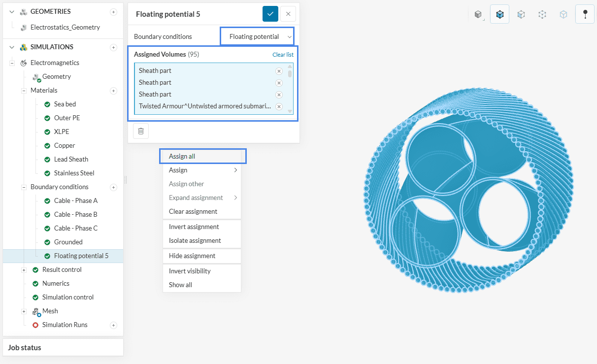
Now, select and hide the remaining volumes such that only the 92 twisted armor cables and the 3 sheath parts are visible.

Add a ‘Floating potential’ boundary condition. Right-click on the Workbench to ‘Assign all’. Make sure all the 95 volumes are added to the assignment.

2.3 Result Control, Numerics and Simulation Control

The Result Control, Numerics and Simulation control for this simulation, are optimized with their default values and need not be altered.

3. Mesh

To create the mesh, we recommend using the Standard mesh algorithm, which is a good choice in general as it is quite automated and delivers good results for most geometries.

In this tutorial, a mesh fineness level of 5 will be used. If you wish to undertake a mesh refinement study, you can increase the fineness of the mesh by sliding the Fineness slider to higher refinement levels or using refinements.

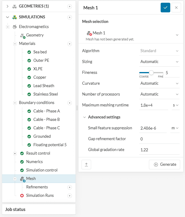
If your mesh settings look the same as in Figure 19, hit the ‘Generate’ button to generate the mesh.

4. Start the Simulation

4.1 Electric Field Strength

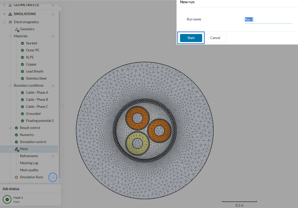
Once mesh is successfully generated, start the simulation. Click on the ‘+’ icon next to Simulation runs. This opens up a dialogue box where you can name your run and ‘Start’ the simulation.

4.2 Capacitance Matrix

While the results from section 4.1 Electric Field Strength are being calculated, you can set up another simulation parallelly to calculate the Capacitance Matrix.

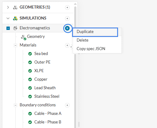
First, click on the options next to the current Electromagnetics simulation tree and select ‘Duplicate’ as follows:

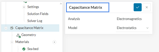
Rename the duplicated simulation to ‘Capacitance Matrix’ and click ‘Save’:

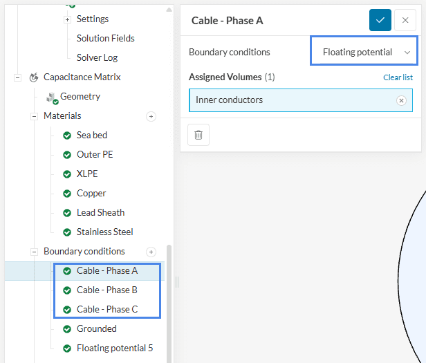
Change the boundary conditions of all three Cables (Phase A, B, and C) to ‘Floating Potential’.

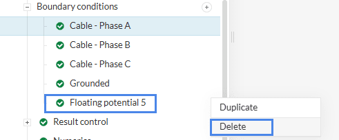
Delete the Floating potential 5 boundary condition.

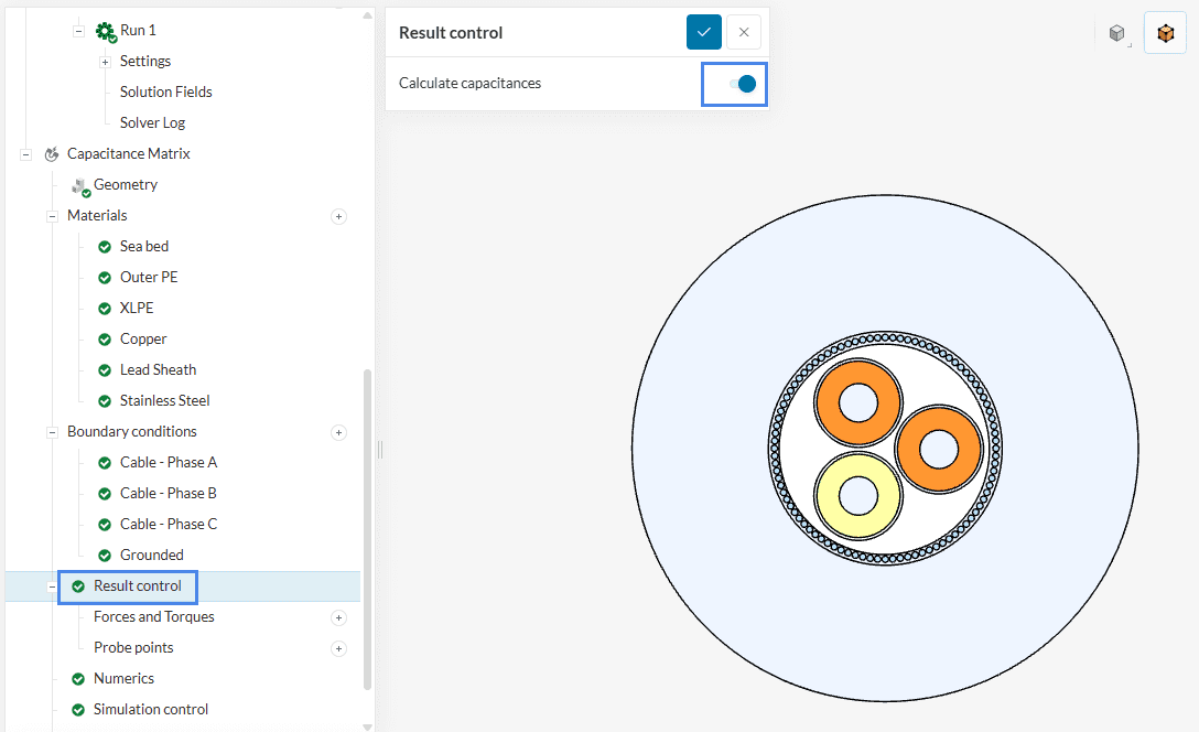
Select ‘Result control’. Toggle on the Calculate capacitances option as shown below:

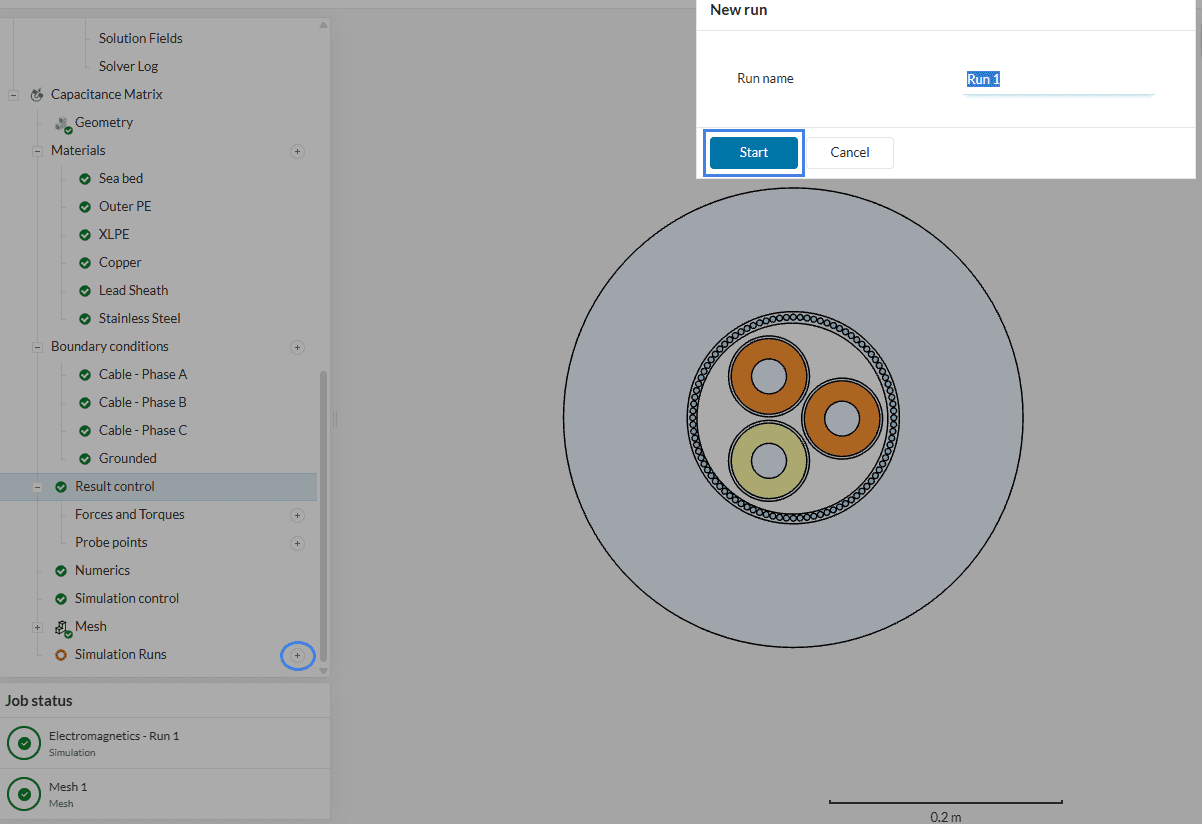
The mesh would already be generated since we duplicated the simulation. Simply start a new simulation run under this tree as follows:

5. Post-Processing

5.1 Electric Field Strength

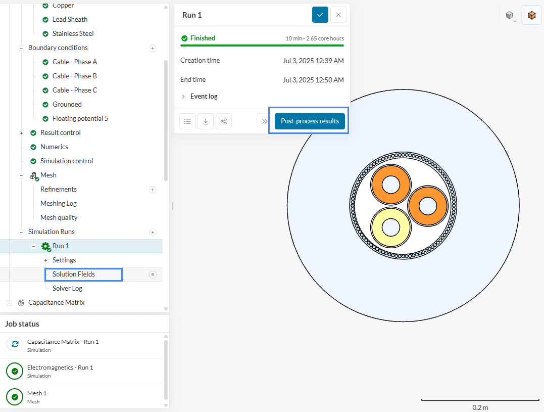
Depending on the instance chosen by the machine, it might take 5-10 minutes for the simulation to finish. Once finished, access the online post-processor of Electromagnetics – Run 1 as indicated in Figure 27.

5.1.1 Electric Field Magnitude

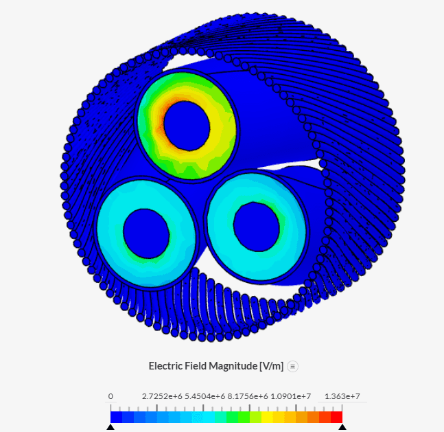
Once inside the post-processor, under the Parts Color filter change Coloring to ‘Electric Field Magnitude’.

• Hit the ‘Cutting Plane’ filter from the top ribbon.
• Adjust the position accordingly and set the orientation of the plane to ‘Z’ axis.
• Adjust Coloring to represent the electric field magnitude
• Toggle on Vectors to visualize the electric field direction.
• Set Scale factor to ‘0.1’ and toggle ‘on’ Project vectors onto plane to visualize the electric field direction.

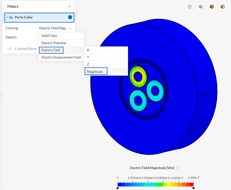
Different parameters can be viewed by changing the coloring.

5.1.2 Electric Potential

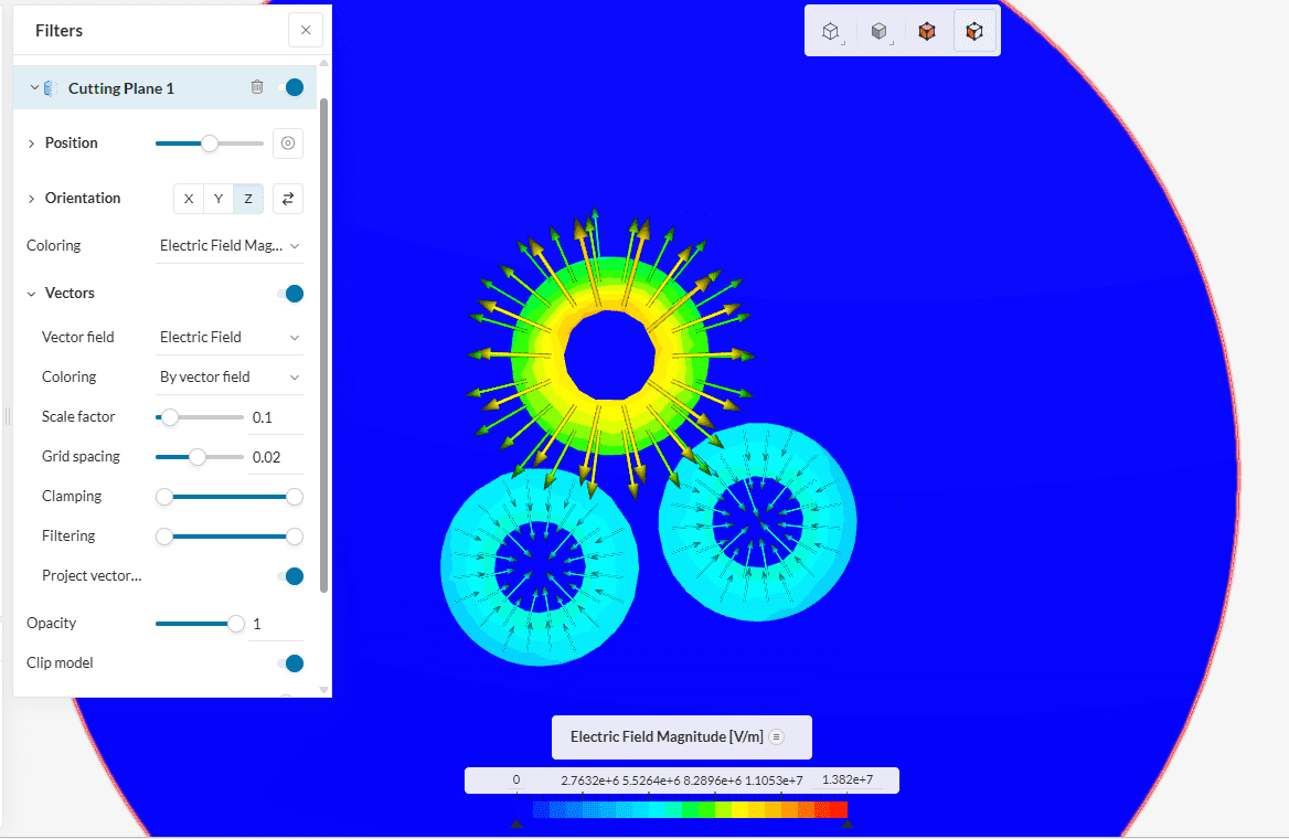
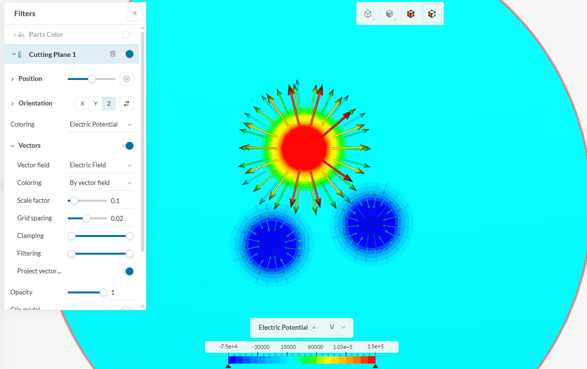
To view the Electric Potential:

Simply set the Coloring of the cutting plane to ‘Electric Potential’.

5.2 Capacitance Matrix

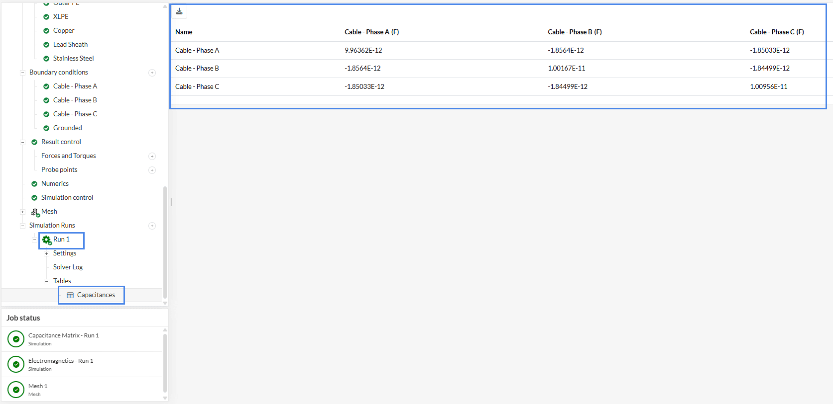
Once the Capacitance Matrix – Run 1 is finished, you can access the capacitance matrix under Tables section of the finished run as follows:

Analyze your results further with the SimScale post-processor. Have a look at our post-processing guide to learn how to use the post-processor.

Last updated: September 3rd, 2025