Centrifugal Force
The centrifugal force boundary condition belongs to solid mechanics applications. More specifically, it can be created in static, dynamic, thermomechanical, frequency, and harmonic analysis types.
This boundary condition is used to apply the forces that act on a structure when it rotates around a fixed axis. It is particularly useful in turbomachinery applications, such as solid mechanics analysis of impellers.
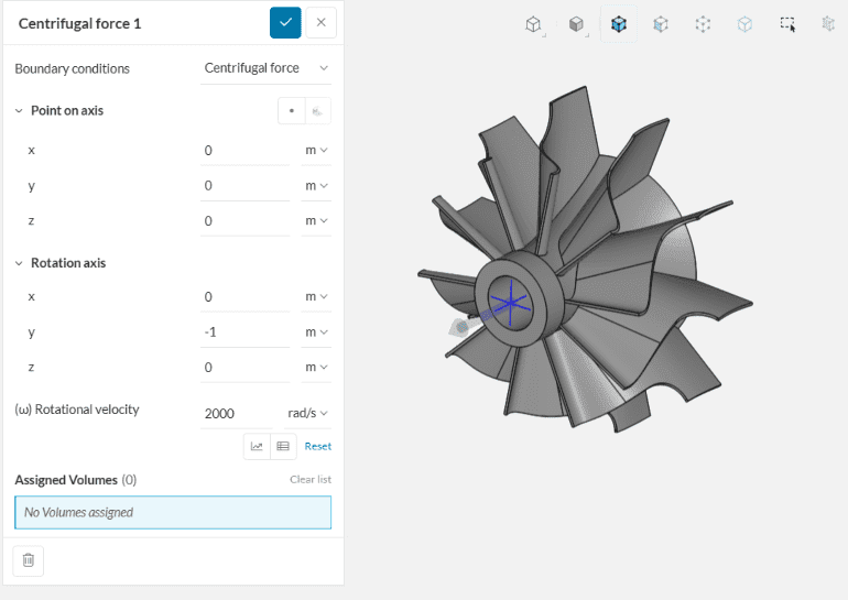
To configure a Centrifugal force boundary condition, the user has to specify:
- A Point on the axis of rotation;
- The Rotation axis direction;
- The Rotational velocity \((\omega)\);
- Lastly, volumes should be assigned to the boundary condition.
Find in Figure 1 the setup window for a centrifugal force boundary condition:
Below we will describe each one of the inputs.
Point on Axis
The user has to define one point on the axis of rotation. Note that the coordinates are given in the global coordinate system.
Therefore, it’s recommended to get accurate point coordinates in a CAD software.
Rotation Axis
The rotation axis is defined by its three components in the global coordinate system. Bear in mind that the resulting direction vector doesn’t need to have a unit length. An arrow in the viewer will display the resulting rotation axis direction.
To determine the direction of the rotation, the right-hand rule applies. The thumb is aligned with the rotation axis, and the other fingers represent the direction of rotation. The direction of rotation can be inverted by prescribing a negative rotational velocity. Taking Figure 1 as a reference we have the following directions of rotation:

Rotational Velocity
The rotational velocity \(\omega\) is given in \(rad/s\) or \(º/s\), as seen in Figure 2. It can be constant or time-dependent (or frequency-dependent, in the case of harmonic analysis). Furthermore, the rotational velocity is supported in parametric experiments. To learn more about this option, make sure to check this article.
Centrifugal Force in Frequency Analysis
Centrifugal forces in frequency analyses are especially useful when evaluating natural frequencies of rotating parts (for example, shafts, pumps, and rotating machinery in general). A volume that is rotating about an axis tends to continue to rotate about the same axis—this phenomenon is named the gyroscopic effect.
By defining a centrifugal force to rotating parts in frequency analysis, the solver is taking the gyroscopic effects into account for the natural frequencies calculation. This way, it is possible to evaluate how the natural frequencies vary for various rotational velocities.
Examples
Find below sample projects that use centrifugal force in the setup:
- Gyroscopic Effects in Frequency Analysis
- Cyclic Symmetric Rotor Under Centrifugal Force
- Harmonic Analysis of Bearing Tolerances of an Impeller
Last updated: January 12th, 2025
Did this article solve your issue?
How can we do better?
We appreciate and value your feedback.


