What Are the Navier-Stokes Equations?
Navier-Stokes equations are partial differential equations that govern the motion of incompressible fluids. These equations constitute the basic equations of fluid mechanics.
The movement of fluid in the physical domain is driven by various properties. For the purpose of bringing the behavior of fluid flow to light and developing a mathematical model, those properties have to be defined precisely to provide a transition between the physical and the numerical domain.
Velocity, pressure, temperature, density, and viscosity are the main properties that should be considered simultaneously when conducting a fluid flow examination. As per physical phenomena, such as combustion, multiphase flow, turbulence, and mass transport, those properties diversify enormously and can be categorized into kinematic, transport, thermodynamic, and other miscellaneous properties\(^1\).
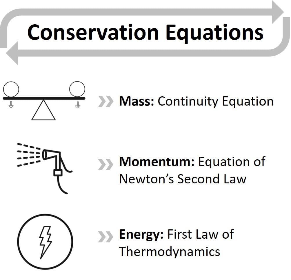
Thermo-fluid incidents directed by governing equations are based on the laws of conservation. The Navier-Stokes (N-S) equations constitute the broadly applied mathematical model to examine changes in those properties during dynamic and/or thermal interactions. The equations are adjustable regarding the content of the problem and are expressed based on the principles of conservation of mass, momentum, and energy\(^1\):
- Conservation of Mass: Continuity Equation
- Conservation of Momentum: Newton’s Second Law
- Conservation of Energy: First Law of Thermodynamics or Energy Equation
Although some sources specify the expression of Navier-Stokes equations merely for the conservation of momentum, some of them also use all equations of conservation of the physical properties. Regarding the flow conditions, the N-S equations are rearranged to provide affirmative solutions in which the complexity of the problem either increases or decreases. For instance, having a numerical case of turbulence according to the pre-calculated Reynolds number requires an appropriate turbulent model to be applied to obtain credible results.
The History of Navier-Stokes Equations
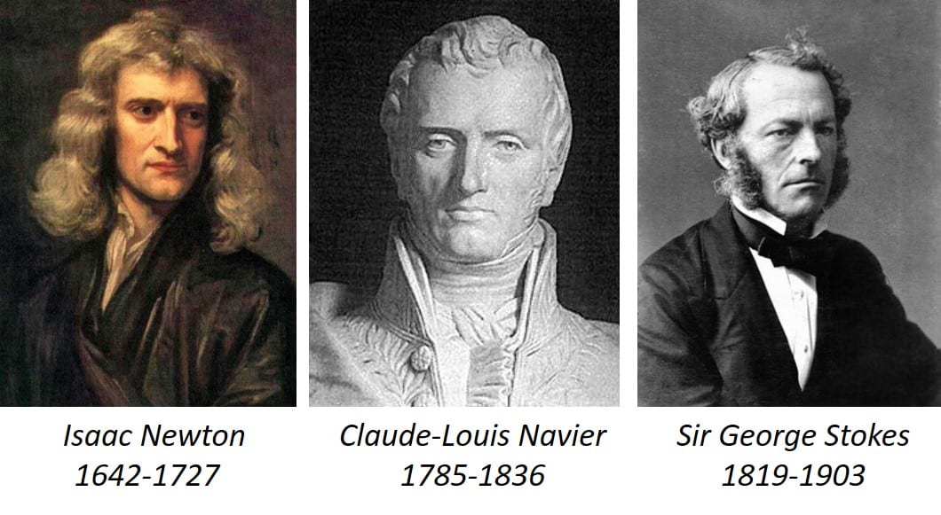
Despite the fact that the motion of fluids is an exploratory topic for human beings, the evolution of mathematical models emerged at the end of the 19th century after the industrial revolution. The initial appropriate description of the viscous fluid motion was indicated in the paper “Principia” by Sir Isaac Newton (1687), in which he investigated the dynamic behavior of fluids under constant viscosity\(^1\).
Later, Daniel Bernoulli (1738) and Leonhard Euler (1755) subsequently derived the equation of inviscid flow, which is now expressed as Euler’s inviscid equations. Even though Claude-Louis Navier (1827), Augustin-Louis Cauchy (1828), Siméon Denis Poisson (1829), and Adhémar St.Venant (1843) had carried out studies to explore the mathematical model of fluid flow, they overlooked the viscous (frictional) force.
In 1845, Sir George Stokes derived the equation of motion of a viscous flow by adding Newtonian viscous terms, thereby the Navier-Stokes Equations were brought to their final form, which has been used to generate numerical solutions for fluid flow ever since\(^{1,2}\).
In short, the Navier-Stokes equations were derived independently and progressively by Claude-Louis Navier and Sir George Stokes over a span of decades in the 19th century. They were based on applying Newton’s second law of motion to fluid flow, taking into account the viscous and pressure effects in order to describe a viscous fluid flow.
Lagrangian vs Eulerian Description of Fluid Motion
The observation method of fluid flow based on kinematic properties is a fundamental issue for generating a convenient mathematical model. The movement of fluid can be investigated with either Lagrangian or Eulerian methods\(^3\).
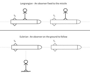
Lagrangian description of fluid motion is based on monitoring a fluid particle that is large enough to detect properties. Between the initial coordinates at time \(t_0\) and coordinates of the same particle at time \(t_1\), millions of separate particles have to be examined through a path that is almost impossible to follow.
In the Eulerian method, no specific particle across the path is followed; instead, the velocity field as a function of time and position is examined. The missile example (Figure 3) precisely fits to emphasize these methods.
The Lagrangian formulation of motion is always time-dependent. As \(a\), \(b\), and \(c\) are the initial coordinates of a particle; \(x\), \(y\), and \(z\) are coordinates of the same particle at time \(t\). Description of motion for Lagrangian:
$$ x=x(a,b,c,\,t),y=y(a,b,c,\,t),z=z(a,b,c,\,t) \tag1$$
In the Eulerian method, \(u\), \(v\) and \(w\) are the components of velocity at the point \((x,y,z)\) while \(t\) is the time. The velocity components \(u\), \(v\) and \(w\) are the unknowns which are functions of the independent variables \(x\), \(y\), \(z\) and \(t\). The description of motion with the Eulerian method for any particular value of \(t\) is:
$$ u=u(x,y,z,\,t),v=v(x,y,z,\,t),w=w(x,y,z,\,t) \tag2$$
The equations of conservation in the Eulerian system in which fluid motion is described are expressed as Continuity Equation for mass, Navier-Stokes Equations for momentum and Energy Equation for the first law of Thermodynamics. The equations are all considered simultaneously to examine fluid and flow fields.
The Three Conservation Equations
Conservation of Mass
The mass in the control volume can be neither created nor destroyed. The conservation of mass states that the mass flow difference throughout the system between the inlet and outlet is zero:
$$ \frac{D\rho}{Dt}+\rho\left(\nabla\cdot\vec{V}\right)=0 \tag3$$
where \(\rho\) is density, \(V\) is velocity and gradient operator \(\nabla\);
$$ \vec{\nabla}=\vec{i}\frac{\partial}{\partial x}+\vec{j}\frac{\partial}{\partial y}+\vec{k}\frac{\partial}{\partial z} \tag4$$
While the density is constant, the fluid is assumed incompressible. Then, continuity is simplified as below, which indicates a steady-state process:
$$ \frac{D\rho}{Dt}=0 \longrightarrow \nabla\cdot\vec{V}=\frac{\partial u}{\partial x}+\frac{\partial v}{\partial y}+\frac{\partial w}{\partial z} =0 \tag5$$
Conservation of Momentum
Momentum describes a mass in motion and is measured as the product between an object’s mass and velocity. As the momentum in a control volume remains constant, the conservation of momentum implies momentum is neither created nor destroyed. It can only change through the action of forces based on Newton’s laws.
The description is set up in accordance with the expression of Newton’s Second Law of Motion:
$$ F=m \times a \tag6$$
where \(F\) is the net force applied to any particle, \(a\) is the acceleration, and \(m\) is the mass. In the case of a fluid, it is convenient to express the equation in terms of the volume of the particle as follows:
$$ \rho\frac{DV}{D_t}=f=f_{body}+f_{surface} \tag7$$
in which \(f\) is the force exerted on the fluid particle per unit volume, and \(f_{body}\) is the applied force on the whole mass of fluid particles as below:
$$ f_{body}=\rho g \tag8$$
where \(g\) is the gravitational acceleration. External forces which are deployed through the surface of fluid particles, \(f_{surface}\) is expressed through pressure and viscous forces as:
$$ f_{surface}=\nabla\cdot\tau_{ij}=\frac{\partial\tau_{ij}}{\partial x_i}=f_{pressure}+f_{viscous} \tag9$$
where \(\tau_{ij}\) is stress tensor. According to the general deformation law of Newtonian viscous fluid given by Stokes, \(\tau_{ij}\) is expressed as\(^2\):
$$ \tau_{ij}=-p\delta_{ij}+\mu\left(\frac{\partial u_i}{\partial x_j}+\frac{\partial u_j}{\partial x_i}\right)+\delta_{ij}\lambda\nabla\cdot V \tag{10}$$
Hence, Newton’s equation of motion can be specified in the form as follows:
$$ \rho\frac{DV}{D_t}=\rho g+\nabla\cdot\tau_{ij} \tag{11}$$
Substitution of equation (10) into (11) results in the Navier-Stokes equations of Newtonian viscous fluid in one equation:
$$ \underbrace{\rho\frac{DV}{Dt}}_{I} = \underbrace{\rho g} _ {II} – \underbrace{\nabla p} _ {III}+\underbrace{\frac{\partial}{\partial x _ i}\left[\mu\left(\frac{\partial v _ i}{\partial x _ j} + \frac{\partial v _ j}{\partial x _ i}\right)+\delta _ {ij} \lambda\nabla\cdot V\right]} \tag{12} _ {IV}$$
\(I\): Momentum convection
\(II\): Mass force
\(III\): Surface force
\(IV\): Viscous force
where static pressure is \(p\) and gravitational force is \(\rho\vec{g}\). Equation (12) is convenient for fluid and flow fields which are both transient and compressible. \(D/Dt\) indicates the substantial derivative as follows:
$$ \frac{D(\,)}{Dt}=\frac{\partial(\,)}{\partial t}+u\frac{\partial(\,)}{\partial x}+v\frac{\partial(\,)}{\partial y}+w\frac{\partial(\,)}{\partial z}=\frac{\partial(\,)}{\partial t}+V\cdot\nabla(\,) \tag{13}$$
If the density of the fluid is constant, the equations are greatly simplified in which the viscosity coefficient \(\mu\) is assumed constant and \(\nabla\cdot V=0\) in equation (12). Thus, the Navier-Stokes equations for an incompressible three-dimensional flow can be expressed as follows:
$$ \rho\frac{DV}{Dt}=\rho g-\nabla p + \mu\nabla^2V \tag{14}$$
For each dimension when the velocity is \(V(u,v,w)\):
$$ \rho\left(\frac{\partial u}{\partial t}+u\frac{\partial u}{\partial x}+v\frac{\partial u}{\partial y}+w\frac{\partial u}{\partial z}\right)=\rho g_x-\frac{\partial p}{\partial x}+\mu\left(\frac{\partial^2u}{\partial x^2}+\frac{\partial^2u}{\partial y^2}+\frac{\partial^2u}{\partial z^2}\right) \tag{15}$$
$$ \rho\left(\frac{\partial v}{\partial t}+u\frac{\partial v}{\partial x}+v\frac{\partial v}{\partial y}+w\frac{\partial v}{\partial z}\right)=\rho g_y-\frac{\partial p}{\partial y}+\mu\left(\frac{\partial^2v}{\partial x^2}+\frac{\partial^2v}{\partial y^2}+\frac{\partial^2v}{\partial z^2}\right) \tag{16}$$
$$ \rho\left(\frac{\partial w}{\partial t}+u\frac{\partial w}{\partial x}+v\frac{\partial w}{\partial y}+w\frac{\partial w}{\partial z}\right)=\rho g_z-\frac{\partial p}{\partial z}+\mu\left(\frac{\partial^2w}{\partial x^2}+\frac{\partial^2w}{\partial y^2}+\frac{\partial^2w}{\partial z^2}\right) \tag{17}$$
\(p\), \(u\), \(v\) and \(w\) are unknowns where a solution is sought by application of both continuity equation and boundary conditions. Besides, the energy equation has to be considered if any thermal interaction is available in the problem — particularly when evaluating convective heat transfer through parameters like the Nusselt number.
Conservation of Energy
Conservation of Energy is the first law of thermodynamics which states that the sum of the work and heat added to the system will result in an increase in the total energy of the system:
$$ dE_t=dQ+dW \tag{18}$$
where \(dQ\) is the heat added to the system, \(dW\) is the work done on the system, and \(dE_t\) is the increment in the total energy of the system. One of the common types of energy equation is:
$$ \rho\left[\underbrace{\frac{\partial h}{\partial t}} _ {I} + \underbrace{\nabla\cdot(hV)} _ {II}\right]=\underbrace{-\frac{\partial p}{\partial t}} _ {III} + \underbrace{\nabla\cdot(k\nabla T)} _ {IV} + \underbrace{\phi} _ {V} \tag{19}$$
where \(h\) is enthalpy and \(k\) is thermal conductivity.
\(I\): Local change with time
\(II\): Convective term
\(III\): Pressure work
\(IV\): Heat flux where
\(V\): Heat dissipation term
Analytical vs Numerical Method Calculations
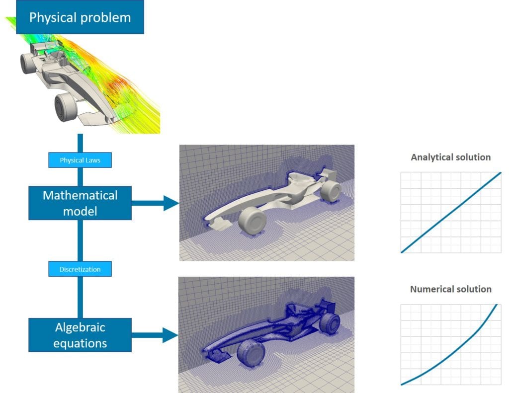
The Navier-Stokes equations have a non-linear structure with various complexities, and thus it is hardly possible to conduct an exact solution for those equations. Consequently, different assumptions are required to grind the equations to a possible solution.
The mathematical model merely gives ties among parameters that are part of the whole process. Hence, the solution of the Navier-Stokes equations can be realized with either analytical or numerical methods.
The analytical method only compensates solutions in which non-linear and complex structures in the Navier-Stokes equations are ignored within several assumptions. It is only valid for simple/fundamental cases such as Couette flow, Poisellie flow, etc\(^3\).
On the other hand, almost every case in fluid dynamics comprises non-linear and complex structures in the mathematical model, which cannot be ignored. Hence, the solutions of the Navier-Stokes equations are carried out within several numerical methods, the omnipresence of Ordinary Differential Equations (ODEs) and Partial Differential Equations (PDEs).
A step-by-step computational analysis of fluid flow can be described as shown in Figure 4.
Time Domain
The analysis of fluid flow can be conducted in either steady (time-independent) or unsteady (time-dependent) conditions. In case the flow is steady, it means the motion of fluid and parameters do not rely on the change in time, the term \(\frac{\partial()}{\partial t}=0\) where the continuity and momentum equations are re-derived as follows:
Continuity equation:
$$ \frac{\partial(\rho u)}{\partial x}+\frac{\partial(\rho v)}{\partial y}+\frac{\partial(\rho w)}{\partial z}=0 \tag{20}$$
The Navier-Stokes equation in \(x\) direction:
$$ \rho\left(u\frac{\partial u}{\partial x}+v\frac{\partial u}{\partial y}+w\frac{\partial u}{\partial z}\right) = \rho g_x-\frac{\partial p}{\partial x}+\mu\left(\frac{\partial^2u}{\partial x^2}+\frac{\partial^2u}{\partial y^2}+\frac{\partial^2u}{\partial z^2}\right) \tag{21}$$
While the steady flow assumption negates the effect of some non-linear terms and provides a convenient solution, the variation of density is still a hurdle that keeps the equation in a complex formation.
Compressibility
Due to the malleable structure of fluids, the compressibility of particles is a significant issue. Despite the fact that all types of fluid flow are compressible in a various range of molecular structures, most of them can be assumed incompressible, in which the density changes are negligible.
Thus, the term \(\frac{\partial\rho}{\partial t}=0\) is thrown away regardless of whether the flow is steady or not, as below:
Continuity equation:
$$ \frac{\partial u}{\partial x}+\frac{\partial v}{\partial y}+\frac{\partial w}{\partial z}=0 \tag{22}$$
The Navier-Stokes equation in \(x\) direction:
$$ \rho\left(\frac{\partial u}{\partial t}+u\frac{\partial u}{\partial x}+v\frac{\partial u}{\partial y}+w\frac{\partial u}{\partial z}\right)=\rho g_x-\frac{\partial p}{\partial x}+\mu\left(\frac{\partial^2u}{\partial x^2}+\frac{\partial^2u}{\partial y^2}+\frac{\partial^2u}{\partial z^2}\right) \tag{23}$$
As the incompressible flow assumption provides reasonable equations, the application of steady flow assumption concurrently enables us to ignore non-linear terms where \(\frac{\partial()}{\partial t}=0\).
Having said that, high-speed flows where the velocity is beyond a critical limit cannot be assumed incompressible. This is determined by the Mach Number (Ma). Mach Number is a dimensionless number that compares the flow velocity with the speed of sound in the surrounding medium. It is calculated as follows\(^3\):
$$ Ma=\frac{V}{a}\ \tag{24}$$
where \(Ma\) is the Mach number, \(V\) is the velocity of flow, and \(a\) is the speed of sound in the flow medium and is a function of its temperature.
- When Mach number is less than 0.3, the flow can be considered incompressible.
- When Mach number is larger than 0.3 – i.e., high-speed flows – the change in density is not negligible, and the flow is considered compressible. For instance, if the velocity of a car is higher than 100\(\frac{m}{s}\), the suitable approach to conducting credible numerical analysis is the compressible flow. Apart from velocity, the effect of thermal properties on the density changes has to be considered in geophysical flows\(^3\).
The Effect of Reynolds Number on Navier-Stokes Equations
Reynolds number (Re) is the ratio of inertial and viscous effects, and it affects the Navier-Stokes equations in truncating the mathematical model. As Reynolds number approaches infinity (\(Re\longrightarrow\infty\)), the viscous effects are presumed negligible, and the viscous terms in Navier-Stokes equations are thrown away.
Therefore, the simplified form of the Navier-Stokes equation, described as the Euler equation, can be specified as follows\(^8\):
The Navier-Stokes equation in \(x\) direction:
$$ \rho\left(\frac{\partial u}{\partial t}+u\frac{\partial u}{\partial x}+v\frac{\partial u}{\partial y}+w\frac{\partial u}{\partial z}\right)=\rho g_x-\frac{\partial p}{\partial x} \tag{25}$$
Even though viscous effects are relatively important for fluids, the inviscid flow model partially provides a reliable mathematical model to predict real processes for some specific cases. For instance, high-speed external flow over bodies is a broadly used approximation, where the inviscid approach reasonably fits. While \(Re\ll1\), the inertial effects are assumed negligible where related terms in Navier-Stokes equations drop out. The simplified form of Navier-Stokes equations is called either creeping flow or Stokes flow\(^8\):
The Navier-Stokes equation in \(x\) direction:
$$ \rho g_x-\frac{\partial p}{\partial x}+\mu\left(\frac{\partial^2u}{\partial x^2}+\frac{\partial^2u}{\partial y^2}+\frac{\partial^2u}{\partial z^2}\right)=0 \tag{26}$$
Having tangible viscous effects, creeping flow is a suitable approach to investigate the flow of lava, swimming of microorganisms, flow of polymers, or lubrication.
Modeling Turbulence Using N-S Equations
The behavior of the fluid under dynamic conditions can be classified as laminar and turbulent. The laminar flow is orderly in that the motion of a fluid can be predicted precisely. The turbulent flow has a chaotic behavior and, therefore, is hard to predict.
The Reynolds number predicts the behavior of fluid flow, whether laminar or turbulent, regarding several properties such as velocity, length, viscosity, and type of flow.
Whilst the flow is turbulent, a proper mathematical model is selected to carry out numerical solutions. Various turbulent models are available in the literature, and each of them has a slightly different structure to examine chaotic fluid flow.
Turbulent flow can be applied to the Navier-Stokes equations to model the chaotic behavior. Apart from the laminar transport quantities of the turbulent flow, it is driven by instantaneous values. Direct numerical simulation (DNS) is the approach to solving the N-S equations with instantaneous values. Having distinct fluctuations varying in a broad range, DNS needs enormous effort and expensive computational facilities.
To avoid those hurdles, the instantaneous quantities are reinstated by the sum of their mean and fluctuating parts as follows:
$$ instantaneous\,value = \overline{mean\,value}+fluctuating\,value’ \tag{27}$$
$$ u = \overline{u}+u’$$
$$ v = \overline{v}+v’$$
$$ w = \overline{w}+w’$$
$$ T= \overline{T}+T’$$
where \(u\), \(v\), and \(w\) are velocity components and \(T\) is temperature. The differences among values are shown in Figure 5 both for steady and unsteady conditions:
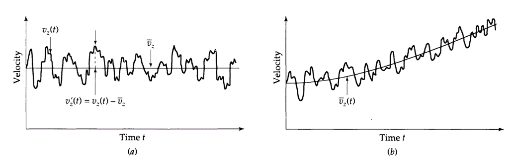
Instead of instantaneous values that cause non-linearity, carrying out a numerical solution with mean values provides an appropriate mathematical model, which is named “The Reynolds-averaged Navier-Stokes (RANS) equation“\(^4\).
The fluctuations can be negligible for most engineering cases. Thus, the RANS turbulence model is a procedure to close the system of mean flow equations. The general form of The Reynolds-averaged Navier-Stokes (RANS) equation can be specified as follows:
Continuity equation:
$$ \frac{\partial\overline{u}}{\partial x}+\frac{\partial\overline{v}}{\partial y}+\frac{\partial\overline{w}}{\partial z}=0 \tag{28}$$
The Navier-Stokes equation in \(x\) direction:
$$ \rho\left(\frac{\partial\overline{u}}{\partial t}+\overline{u}\frac{\partial\overline{u}}{\partial x}+\overline{v}\frac{\partial\overline{u}}{\partial y}+\overline{w}\frac{\partial\overline{u}}{\partial z}\right)=\rho g_x-\frac{\partial\overline{p}}{\partial x}+\mu\left(\frac{\partial^2u}{\partial x^2}+\frac{\partial^2u}{\partial y^2}+\frac{\partial^2u}{\partial z^2}\right) \tag{29}$$
The turbulence model of RANS varies in regard to methods such as k-omega, k-epsilon, k-omega-SST, and Spalart-Allmaras. Likewise, Large Eddy Simulation (LES) is another mathematical method for turbulent flows which is also comprehensively applied for several cases. Robust LES ensures more accurate results than RANS but requires much more time and computer memory. As in DNS, LES resolves the larger eddies but models the smaller ones\(^4\).
The simple form of the Navier-Stokes equations only encompasses the change in properties such as velocity, pressure, and density under dynamic conditions for one phase laminar flow. Most engineering applications require further mathematical models for numerical simulation. Some common engineering problems and their relevant mathematical models are shown below:
- Airflow in a duct: Single phase flow, laminar/turbulent, steady/unsteady
- Water flow in an open channel: Multiphase flow, laminar/turbulent, steady/unsteady
- Combustion in cylinder: Multiphase flow, laminar/turbulent, unsteady, chemical reaction, heat transfer, mass transfer
- Condensation/evaporation of water: Multiphase flow, laminar/turbulent, unsteady, heat transfer, mass transfer
Navier-Stokes Equations in Microfluidics
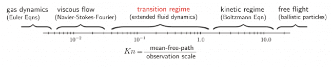
The Navier-Stokes equations cannot compensate for the physical model of the flow at very small scales, such as the motion of single bacteria — also called microfluidics. Thereby, it is convenient to either change or reinstate the Navier-Stokes model with a suitable mathematical model.
The Knudsen number (Kn) is a dimensionless number that is the ratio of the mean free path of molecular structure to the observation scale. The preferred model in accordance with the Knudsen number is shown in Figure 6:
Real-Time Simulation
The Navier-Stokes equations have been considered crucial even in the animation/video game world\(^5\). For the purpose of generating a real-time animation, the application of these equations provides stunning results, enhancing reality\(^6\). They are the reason why modern video games appear to be realistic in many more ways than several years ago. Just think about the movement of flags in the wind: doesn’t this look absolutely realistic in modern games?!

References
- White, Frank (1991).Viscous Fluid Flow. 3rd Edition. McGraw-Hill Mechanical Engineering. ISBN-10: 0072402318.
- Stokes, George (1851). “On the Effect of the Internal Friction of Fluids on the Motion of Pendulums”. Transactions of the Cambridge Philosophical Society. 9: 8–106.
- White, Frank (2002). Fluid Mechanics. 4th edition. McGraw-Hill Higher Education. ISBN: 0-07-228192-8.
- Cebeci, T., Shao, J.P., Kafyeke, F., Laurendeau, E (2005). Computational Fluid Dynamics for Engineers. Horizon Publishing Inc. ISBN: 0-9766545-0-4.
- https://www.dgp.toronto.edu/people/stam/reality/Research/pdf/GDC03.pdf
- https://software.intel.com/en-us/articles/fluid-simulation-for-video-games-part-1
- https://www.mathcces.rwth-aachen.de/2research/0mms/0gases/start
- Bird, R.B., Stewart, W.E. and Lightfoot, E.N. (2001). Transport Phenomena, 2th edition. John Wiley Sons. ISBN 0-471-41077-2.
- https://en.wikipedia.org/wiki/Isaac_Newton
- https://en.wikipedia.org/wiki/Claude-Louis_Navier
- https://en.wikipedia.org/wiki/Sir_George_Stokes,_1st_Baronet
Last updated: March 16th, 2026
Did this article solve your issue?
How can we do better?
We appreciate and value your feedback.
What's Next
What is Reynolds Number?

