Documentation
Viscosity is an intensive property of a fluid that measures its internal resistance to motion or deformation. It plays an important role in areas such as aerodynamics and reservoir engineering since it determines the nature of the flow of a given fluid, such as air, water or oil.
A tangible everyday example of the comparison between two fluids’ viscosities is the one between honey and milk. Intuitively, honey is more viscous than milk. This can be seen in an experiment such as the one in Figure 1 below, where the viscous fluid (right) is more difficult to flow than the less viscous fluid (left).

The most basic ideas of the mathematics of fluid mechanics — including its structure and formulations — emerged between the late seventeenth century and the first half of the eighteenth century. More advanced and involved concepts such as turbulence, discontinuities, and viscosity were introduced in the nineteenth and twentieth centuries.
The field of fluid dynamics was first scientifically defined in Newton’s Principia Mathematica in 1687, analyzing for the first time the dynamics of fluids. Newton’s law of viscosity described the relationship between a fluid’s shear stress and shear rate when subjected to mechanical stress. However, Newton treated fluids such as air as a particle agglomerate. It was only with Leonhard Euler that the differential and continuum form of fluid dynamics was developed
It was before Newton, though, that many important questions began to appear. Christiaan Huygens was interested in studying the effects of bodies inside fluids. He was a student of ballistics and, therefore, studied how air resistance worked. The problem of determining the dynamics of a body in relative motion — with a fluid surrounding it — is represented through the problem of resistance and was, in many aspects, intrinsically related to the study of viscosity.
Viscosity is a critical property when studying fluid motion. It helps determine the loss of friction between adjacent fluid layers due to the shear energy in the fluid. In other words, viscosity determines the internal resistance of the fluid to motion. A fluid with higher viscosity is more resistant to motion than a less-viscous fluid. Take oil, for example, which is more viscous than water.
The mathematical models of fluid dynamics are mainly based on mass conservation, momentum balance, and energy conservation, together with the constitutive relations of the fluid. When coupled, the above conservation principles can form the Navier-Stokes equation, which is used to describe the motion of many viscous fluids.
The mass conservation can be stated as follows:
where
The momentum conservation can be written as
where
These equations form the Navier-Stokes system. It’s common to approximate
In general, when considering incompressible flow, where the fluid is not compressed or expanded rapidly,
In this case,
Consequently, for incompressible or isochoric flow, assuming
This system is known as the incompressible Navier-Stokes system.
As can be seen from the above equations, viscosity plays an important role in the determination of the dynamics of a fluid. From the incompressible Navier-Stokes equations, it follows that viscosity is the diffusion coefficient associated with the Laplacian of the velocity.
There are several types of viscosity. The most commonly used in the field of fluid dynamics is the shear — or dynamic viscosity — represented here as
When dealing with shock waves and phenomena that include high and rapid compression of the fluid, the bulk viscosity
One common expression that uses kinematic viscosity is the Reynolds number. It relates momentum to the viscous forces of a fluid.
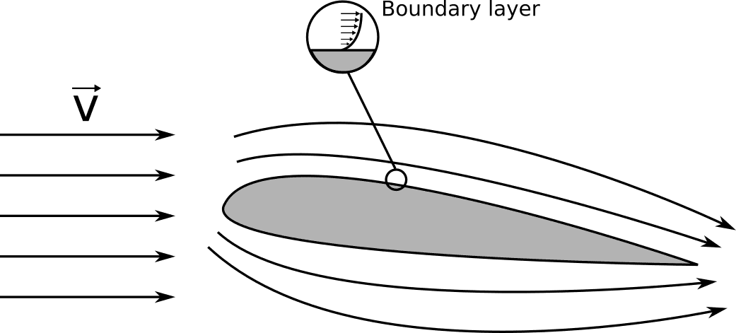
The shear or dynamic viscosity is commonly obtained with a velocity profile experiment. One of the most important examples of a velocity profile is the one in a boundary layer, as is shown in Figure 2 below, adapted from
The section of a body, such as a wing, is represented in a current flow. The boundary layer is the region where viscosity effects are most significant in body-fluid interactions.
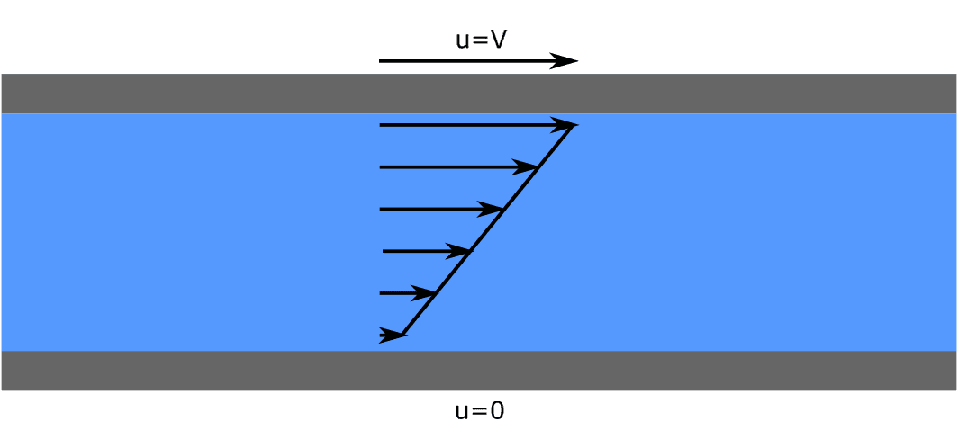
A famous velocity profile experiment involves two parallel and sufficiently large plates with a non-zero relative tangential velocity, zero normal velocity, and a fluid between the two plates. For simplicity, the experiment is made such that one plate is fixed while the other moves tangentially with a tangential velocity
A velocity profile would then appear in the fluid. The fluid in contact with the fixed plate would have zero velocity, while the fluid in contact with the moving plate would have the same velocity as the plate’s, namely
For a Newtonian fluid, where the rate of deformation is linearly proportional to the shear stress, the shear viscosity in a 1D flow can be expressed as follows
where
In regions not close to solids, it is common to neglect viscous forces since inertial and pressure forces dominate in those regions. These regions are called inviscid flow regions. When in inviscid regions, it is common to adopt the Euler system, which models the motion of an inviscid fluid as:
The Navier-Stokes equations above are derived considering a linear relationship between the shear stress and the velocity gradient in the momentum balance equation. The mathematics for non-Newtonian fluids can become extremely involved, though.
In such cases, the viscosity will be some function of the velocity. The field of rheology studies the flow of non-Newtonian fluids and many other models for viscosity
In the case of non-Newtonian flow, the ratio
For example, a fluid for which the apparent viscosity increases with the rate of deformation is called a dilatant fluid, while a fluid for which the apparent viscosity decreases with the rate of deformation is called a pseudoplastic fluid.
The SimScale public projects library provides a number of computational experiments that explore the nature of viscous flows. Here are some simulation examples to explore.
Beginning with the no-slip condition, Figure 4 below shows the cross-section velocity profile inside a relatively long pipe. It can be noticed that the velocity at the boundary is zero.
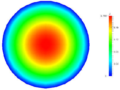
Explore this pipe flow simulation project in more detail.
Figure 5 shows a compressible airflow, which analyzes an airfoil, demonstrating the capability of SimScale when dealing with compressible flows.

Explore this compressible, transient airfoil simulation in more detail.
A common non-Newtonian fluid is blood. SimScale features projects simulating blood flow.
The following project simulates the blood flow inside an artery bifurcation and compares three blood vessel cases: one healthy, one moderately blocked, and one severely blocked.
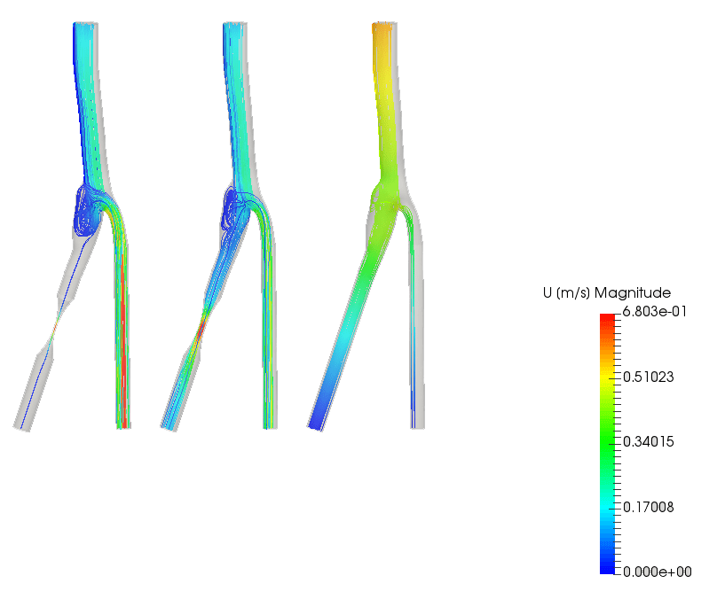
Explore this simulation project of blood flow in a carotid artery bifurcation in more detail.
If there is one thing we love in Germany, it is beer. This is why we could not resist and simulated pouring ourselves one liter of beer in a Maßkrug. In the simulation below, you can see the velocity of the beer, which is why you’ll only see a layer moving up the Krug.
References
Last updated: August 11th, 2023
We appreciate and value your feedback.
What's Next
What is Laminar Flow?Sign up for SimScale
and start simulating now