Documentation
With the variable time step feature, users can manually enter a series of time steps to optimize their transient simulations. For example, start with a fine time step to accurately capture the initial transient behavior, and then increase the time step as the simulation progresses towards convergence. By setting a coarser time step later in the simulation, one can achieve faster results and save computational resources.
As is obvious, this feature is only available for transient multi-purpose simulations.
Under the Simulation control item in the simulation tree, the settings panel is as depicted in Figure 1:
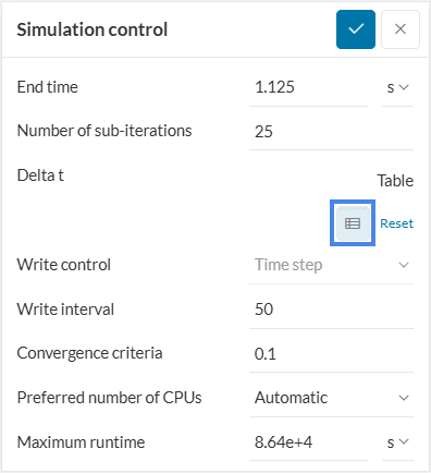
On clicking the table icon, the following panel appears:
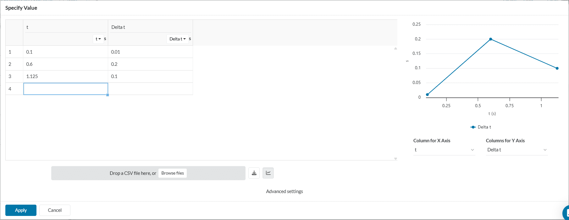
The explanation for the above example is as follows:
| Time | Time step | Calculated time steps |
| 0.1 | 0.01 | [0, 0.01, 0.02, 0.03, 0.04, 0.05, 0.06, 0.07, 0.08, 0.09, 0.1] |
| 0.6 | 0.2 | [0.3, 0.5, 0.6] |
| 1.125 | 0.1 | [0.6, 0.7, 0.8, 0.9, 1, 1.1, 1.125] |
For the time 0 to 0.1 seconds, the time step defined is 0.01 seconds. The calculated time steps are derived using the formula:
$$Calculated\ time\ steps = \frac{Time} {Time\ step}$$
In a similar fashion, a time step of 0.2 seconds is used as the simulation continues from 0.1 seconds to 0.6 seconds. This process continues until the end time of 1.125 seconds.
Important
For each simulation duration, the end time is respected irrespective of the defined time step. Every consequent run will start from the end of the previous run’s duration. For e.g., row 2 in Table 1 calculates the time step 0.6 despite being just 0.1 seconds time step away from 0.5. Similar behavior is observed in row 3 with the time step 1.125, and the simulation stops.
Continuing from the above example, a typical simulation result control plot with varying time steps would look as follows:
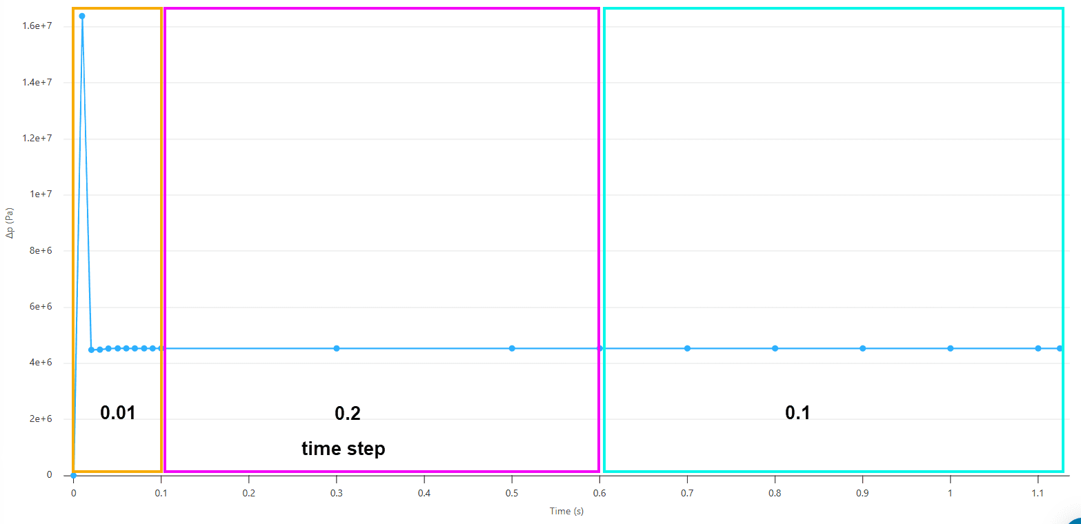
The Pressure difference plot against time in Figure 3 visually depicts the same concept as explained in Table 1.
Last updated: September 9th, 2025
We appreciate and value your feedback.
Sign up for SimScale
and start simulating now