Local Coordinate Systems

Local Coordinate Systems (LCS) allow you to define custom reference frames for your simulation setup. Instead of specifying boundary condition values — such as forces, displacements, or material properties — relative to the global coordinate system, you can create local coordinate systems and apply values relative to them. This is especially useful for models with cylindrical symmetry, angled features, or any geometry where the global axes do not align naturally with the directions of interest.

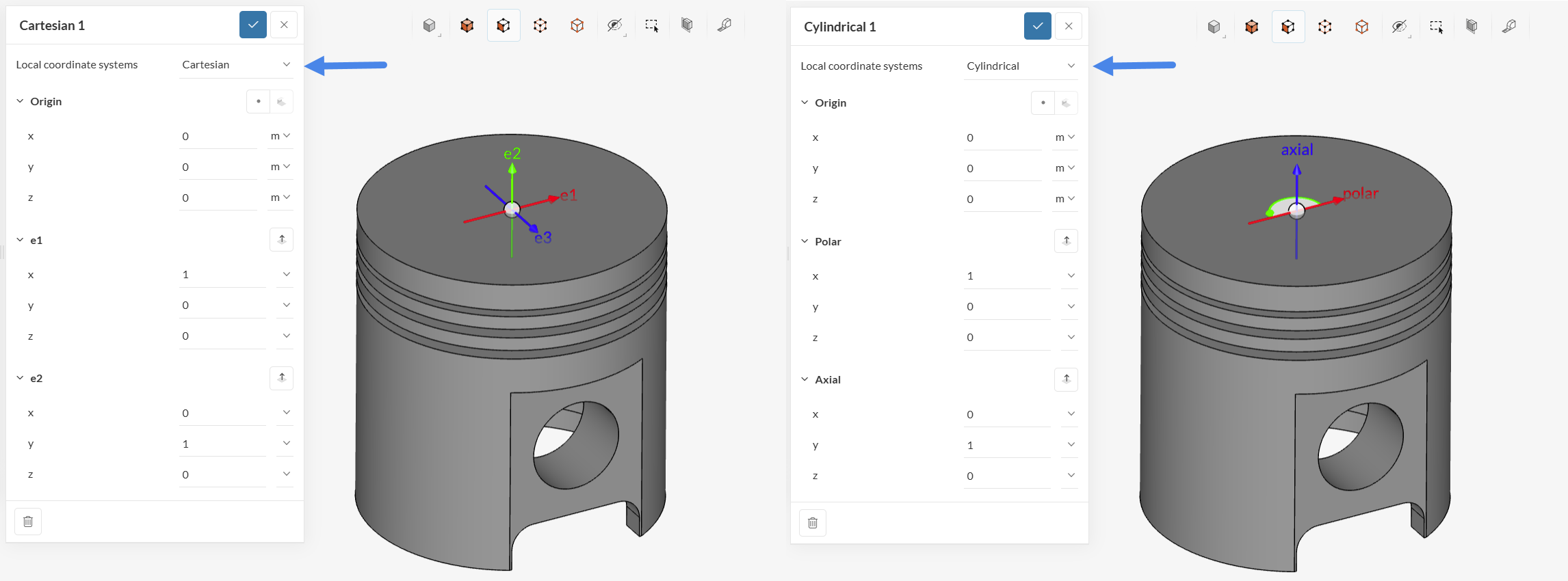
SimScale supports two types of local coordinate systems:

Cartesian — defined by an origin point and two axis vectors (e1 and e2)
Cylindrical — defined by an origin point, a polar axis (e1), and a longitudinal axis (e3)

Figure 1: Global vs. Local Coordinate Systems. A comparison between the default global reference frame (x, y, z) and a custom local coordinate system (e1, e2, e3) aligned with the geometry of the connecting rod.

Creating a Local Coordinate System

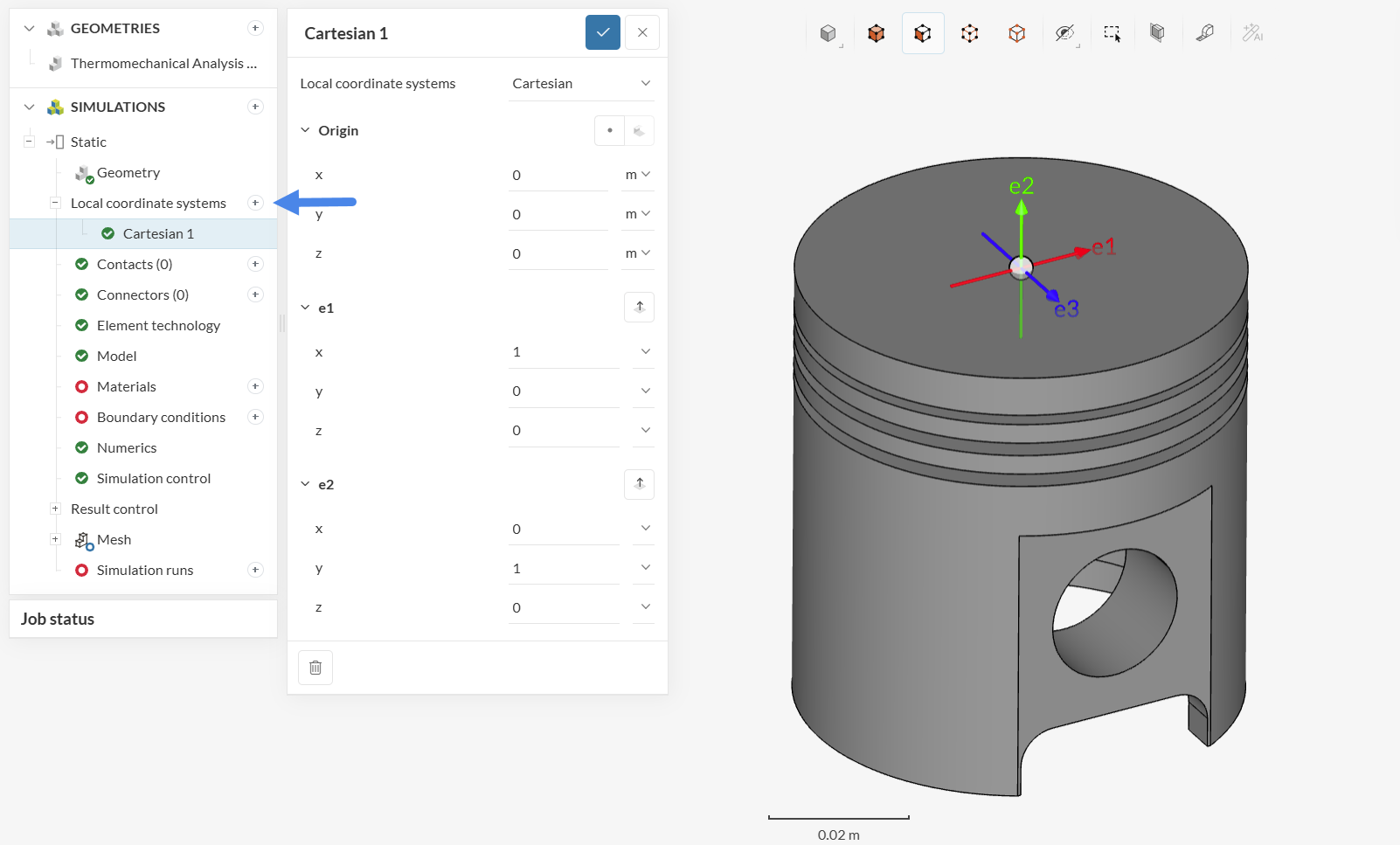
If the active analysis type supports local coordinate systems, a Local coordinate systems node appears in the simulation tree. To create a new coordinate system:

Click the + icon on the Local coordinate systems node.
A new coordinate system is created with default values and added to the tree.
Configure the coordinate system in the settings panel on the right.

Creating a local coordinate system — Figure 2: Creating local coordinate system.

Coordinate System Settings

Each local coordinate system has a user-defined Name (defaulting to “Coordinate System N+1”) and a Type: either Cartesian (default) or Cylindrical.

Cartesian Coordinate System

Property	Description	Default
Origin	The origin point of the coordinate system	(0, 0, 0)
e1	Vector defining the first axis	(1, 0, 0)
e2	Vector defining the second axis	(0, 1, 0)

The third axis (e3) is computed automatically as the cross product of e1 and e2 and does not need to be specified.

Cylindrical Coordinate System

Property	Description	Default
Origin	The origin point of the coordinate system	(0, 0, 0)
e1	The polar axis — defines the zero azimuth direction	(1, 0, 0)
e3	The longitudinal axis — the axis of the cylinder	(0, 0, 1)

Setting the Origin and Axes

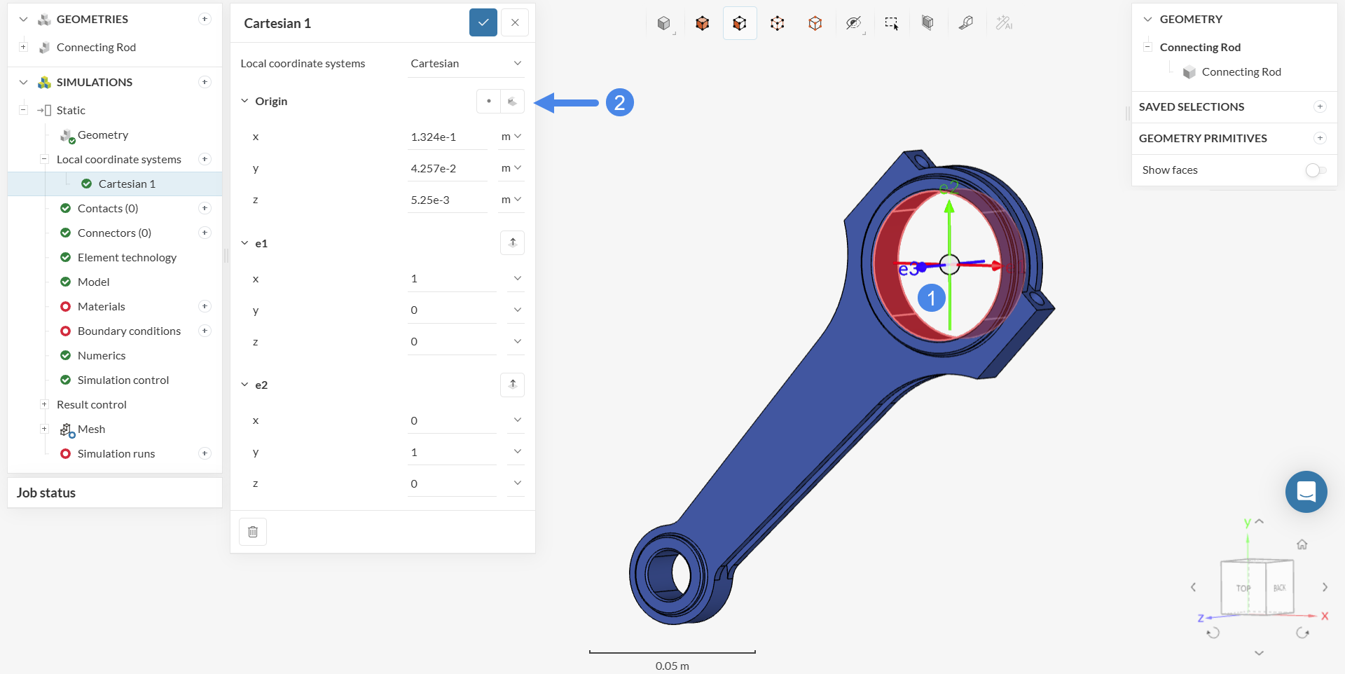
All values can be entered manually. The viewer also provides two interactive tools to speed up the setup:

Pick point from the viewer and Select entity to enable center picking — for setting the origin by clicking a point or face center in the 3D viewer as shown in Figure 4.
Pick face normal from the viewer — for setting an axis direction by clicking a face to use its normal vector. As shown in Figure 5, first click on the pick face normal icon, then select the face.

Figure 4: Use point and entity selection to define the origin of the coordinate system.

Pick face normal from the viewer — Figure 5: Use the pick face normal to orient the axis of the coordinate system.

Axis Validation

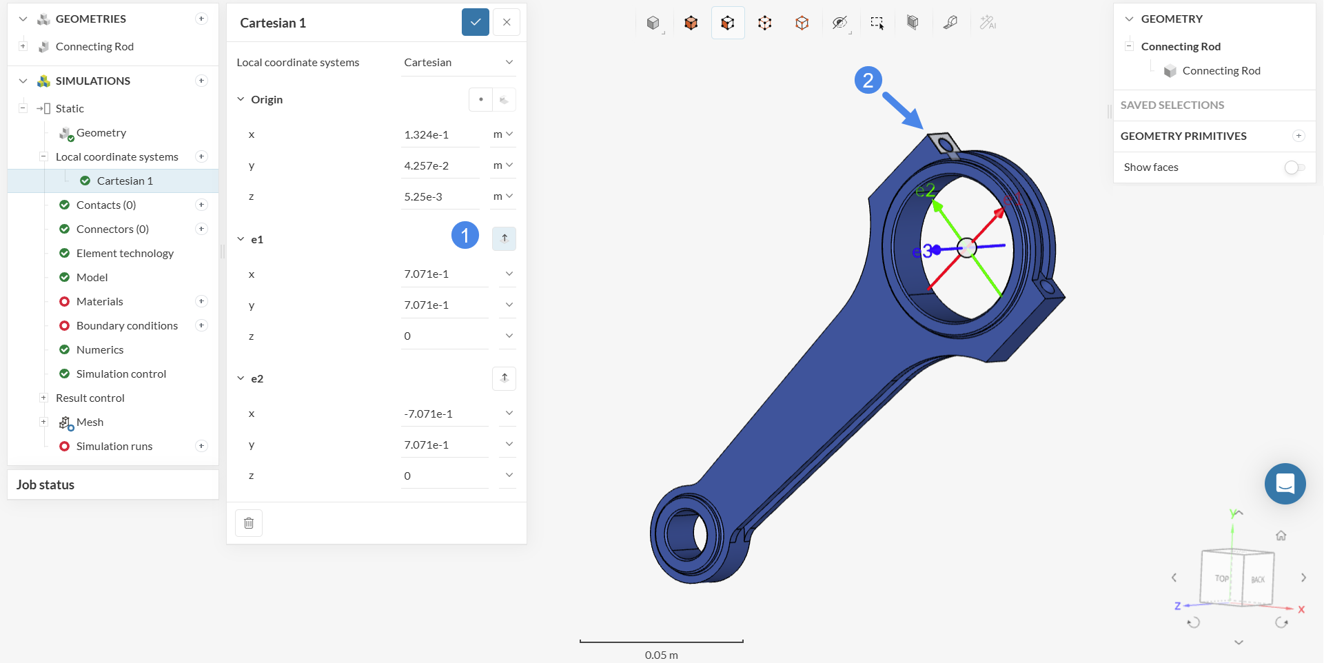
Axis vectors do not need to be unit vectors — any magnitude is accepted. SimScale applies the following rules when the coordinate system is saved:

Condition	Result
Vectors are perpendicular	Valid — normalized and used as defined
Vectors are not perpendicular but not co-linear	Valid — automatically orthogonalized to produce a right-handed frame
Vectors are co-linear	Validation error: “Vectors defining the coordinate system must not be co-linear.” The coordinate system cannot be used until corrected

Visualization

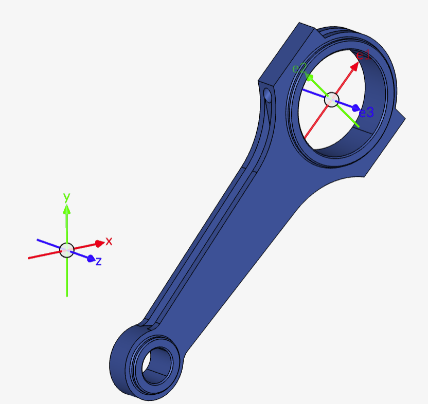
Local coordinate systems are displayed in the 3D viewer using colored arrows:

Cartesian — three arrows from the origin, colored red (e1), green (e2), and blue (e3)
Cylindrical — a red arrow for the polar axis (e1), a blue arrow for the longitudinal axis (e3), and a curved arc indicating the angular direction

Figure 6: Cartesian coordinate system is composed of 3 arrows (left) and the Cylindrical two arrows and one arc (right)

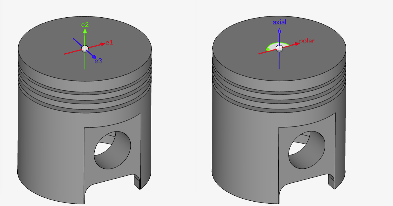
Arrow lengths are scaled automatically based on the size of the model. If the coordinate system definition is invalid (co-linear vectors), no arrows are displayed.

The global coordinate system is always shown in the viewer. A local coordinate system is displayed when it is selected in the tree or when a boundary condition using it is open. You can toggle the visibility of all coordinate systems using the Show/Hide option in the viewer toolbar.

Using Local Coordinate Systems

After creating a custom reference frame, you can assign it to specific physics definitions to simplify your setup. Local coordinate systems can be applied across three main areas of your simulation: boundary conditions, material properties, and advanced tabular inputs.

In Boundary Conditions

Boundary conditions that support local coordinate systems include a Coordinate system type field with two options:

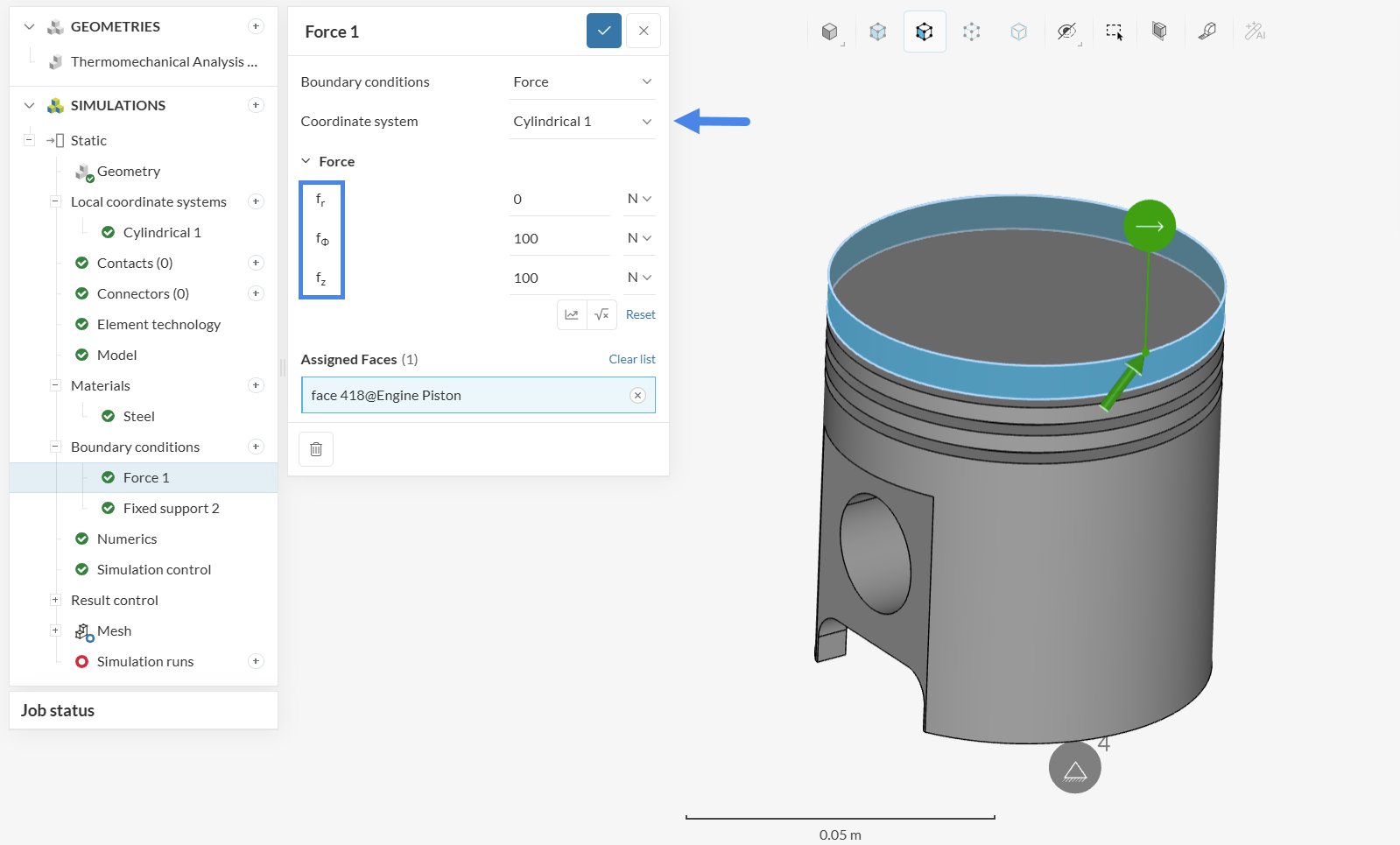
Global (default) — values are specified in the standard global reference frame
Local — a second field, Local coordinate system, appears as a dropdown listing all defined local coordinate systems. Select one or choose + New coordinate system to create one inline

As shown in Figure 7 above, when a local coordinate system is assigned, the component labels in the boundary condition update to reflect the selected frame. The table below details these label changes:

Value type	Cartesian labels	Cylindrical labels
Vector (e.g. force, displacement)	Fx, Fy, Fz	F_radial, F_tangential, F_axial
Position (e.g. point)	x, y, z	r, φ, z

Note

One coordinate system applies to all values within a single boundary condition. For example, in a Remote Displacement boundary condition, the displacement, rotation, and external point all reference the same coordinate system.

In Materials

Orthotropic material properties can be defined relative to a local coordinate system. When a cylindrical LCS is assigned, the material property labels update to reflect radial, tangential, and axial directions (for example, Young’s Modulus in each direction).

In Tables and Expressions

When defining boundary conditions using tabular or expression input with a cylindrical coordinate system, the independent variables change from Cartesian (X, Y, Z, T) to cylindrical (R, φ, Z, T), and the dependent variables use radial, tangential, and axial components.

Important

When using cylindrical coordinates in tables or expressions, the angular variable φ must be specified in radians, not degrees.

Managing Local Coordinate Systems

Select a coordinate system in the simulation tree to edit its values. When editing, a warning is shown:

This coordinate system might be in use in your simulation setup. Editing it will affect your setup. Please be sure before you save or discard your changes.

Use the save and discard buttons in the top right of the panel to confirm or cancel changes.

To duplicate or delete a coordinate system, click the menu icon (⋮) on the coordinate system entry in the tree and select the desired action.