Validation Case: Taylor-Couette Flow
The Taylor-Couette flow validation case belongs to fluid dynamics. This test case aims to validate the following parameters:
- Rotating wall
- Velocity profile
- Pressure profile
SimScale’s simulation results were compared to analytical results obtained from methods elucidated in the Scholarpedia article on Taylor-Couette flow\(^1\).
Geometry
The so-called Taylor-Couette flow occurs in the gap between two infinitely long concentric cylinders, when at least one of them is rotating. Therefore, the geometry for this project consists of a slice of an annulus between two cylinders, as seen in Figure 1:
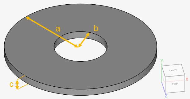
The dimensions of the geometry are given in Table 1:
| Geometry parameters | Dimension \([m]\) |
| Outer radius (a) | 1 |
| Inner radius (b) | 0.35 |
| Thickness of the slice (c) | 0.1 |
Analysis Type and Mesh
Tool Type: OPENFOAM®
Analysis Type: Steady-state incompressible flow
Turbulence Model: Laminar
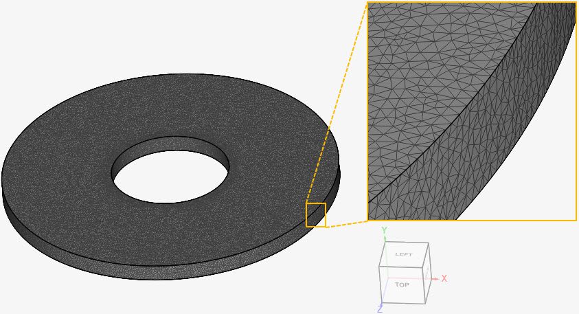
Mesh and Element Types: The mesh used in this case was created in SimScale with the standard algorithm.
Find in Table 2 an overview of the resulting mesh:
| Case | Mesh Type | Cells | Element Type |
| Taylor-Couette flow | Standard | 488457 | 3D tetrahedral/hexahedral |
Find below the standard mesh used for this case:
Simulation Setup
Material:
- Viscosity model: Newtonian;
- \((\nu)\) Kinematic viscosity: 1e-5 \(m²/s\);
- \((\rho)\) Density: 1 \(kg/m^3\).
Boundary Conditions:
Before defining the boundary conditions, the current nomenclature will be used for the rest of this documentation:
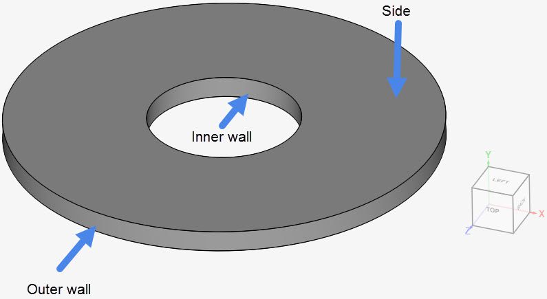
In the table below, the configuration for both velocity and pressure are given at each of the boundaries:
| Nomenclature | Boundary Type | Velocity | Pressure |
| Inner wall | Custom | Rotating wall: 0.001 \(rad/s\) around the positive y-axis | Zero gradient |
| Outer wall | Custom | Fixed value: 0 (no-slip condition) | Zero gradient |
| Sides | Custom | Symmetry | Symmetry |
Reference Solution
The analytical solution\(^1\) for Taylor-Couette flow is computed from the simplified Navier-Stokes in cylindrical coordinates. Before calculating the velocity and pressure profiles, we need to calculate two constants, \(A\) and \(B\):
$$A = \frac {\omega_{out}R_{out}^2-\omega_{in}R_{in}^2}{R_{out}^2-R_{in}^2} \tag {1}$$
$$B = (\omega_{in} – \omega_{out})R_{out}^2\frac {R_{in}^2}{R_{out}^2-R_{in}^2} \tag{2}$$
where:
- \(\omega_{in}\) and \(\omega_{out}\) \([rad/s]\) are the rotational velocities of the inner and outer walls, respectively;
- \(R_{in}\) and \(R_{out}\) \([m]\) are the inner and outer walls’ radius.
The resulting velocity profile \(U\) is a function of radius \(r\). The equation is given below:
$$U(r) = Ar + \frac {B}{r} \tag {3}$$
Similarly, for pressure \(P\):
$$P(r) = A^2\frac {r^2}{2}+2ABln(r)-\frac {B^2}{2r^2} \tag {4}$$
Result Comparison
The velocity and pressure variation in the radial direction obtained with SimScale are compared to the analytical solution.
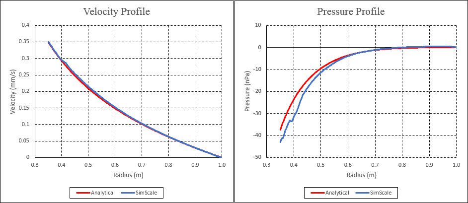
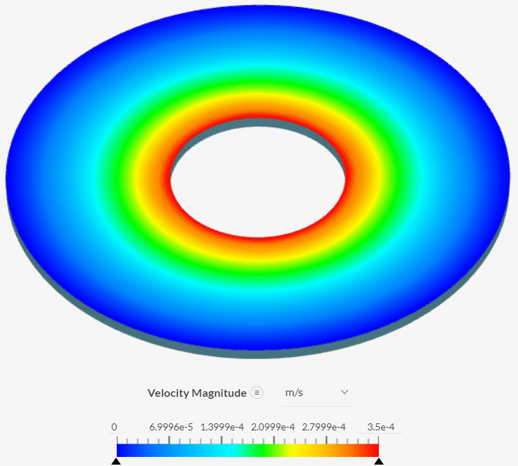
In Figure 5, we can see the velocity profile due to the rotation of the inner wall.
References
Last updated: February 16th, 2026
Did this article solve your issue?
How can we do better?
We appreciate and value your feedback.


