Tutorial: Hex-dominant Parametric Meshing of a Front Wing
This documentation provides a step-by-step tutorial for a mesh creation of an F1 front wing model, using the “Hex-dominant parametric” approach. The “Hex-dominant parametric” (only for CFD) is the semi-automatic meshing option that uses hexahedral cells and allows full flexibility in meshing parameters with all types of refinement options. The objective is to get a high-quality mesh with sufficient resolution to capture key features in the model.
This tutorial will highlight some essential points of the meshing process that help users achieve better simulation results.
Overview
This tutorial teaches how to:
- Use SimScale’s Geometry Operation features.
- Get a new simulation started.
- Mesh with the SimScale Hex-dominant parametric algorithm.
We are following the typical SimScale workflow:
- Preparing the CAD model for the simulation
- Setting up the simulation
- Creating the mesh
If you want to learn more about the Hex-dominant parametric algorithm, take a look at this document: Main Settings for Hex-dominant parametric.
Please Note!
- This is a tutorial purely about meshing. There will not be any simulation performed.
- The Hex-dominant algorithm is an advanced mesher. If you are new to SimScale and just getting started we highly recommend to use the standard mesher.
1. Prepare the CAD Model and Select the Analysis Type
1.1. Import the CAD Into Your Workbench
First of all, click the button below. It will copy the tutorial project containing the geometry into your own Workbench.
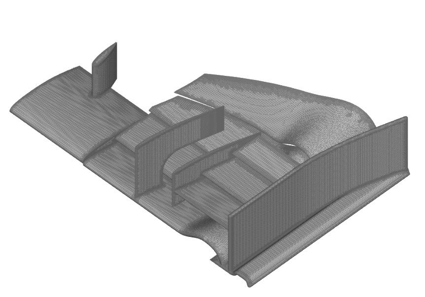
The following picture demonstrates what should be visible after importing the tutorial project.
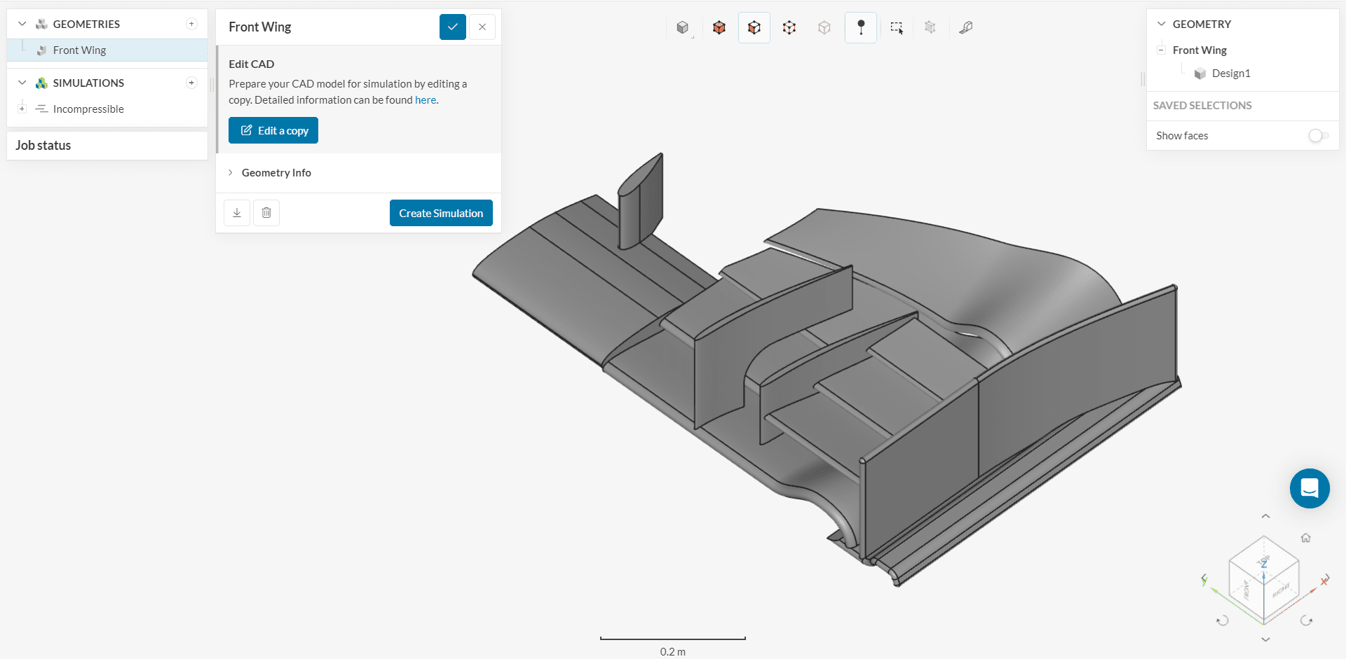
1.2. Create the Simulation
After the CAD is imported, click on the ‘Create Simulation’ option.
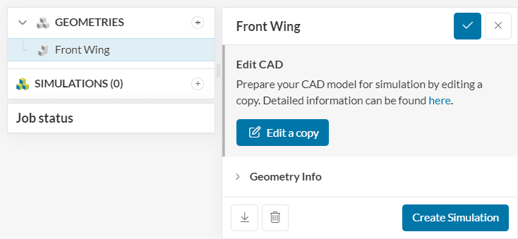
Choose ‘Incompressible fluid flow’ as the analysis type.
2. Mesh
Be Aware
The boundary conditions for cases where the mesh is created with the hex-dominant parametric are assigned on the faces of the generated mesh. For the rest of the meshing algorithms, the assignment takes place on the faces of the model. As a result, for each new mesh with the hex-dominant parametric, the user has to define the boundary conditions again.
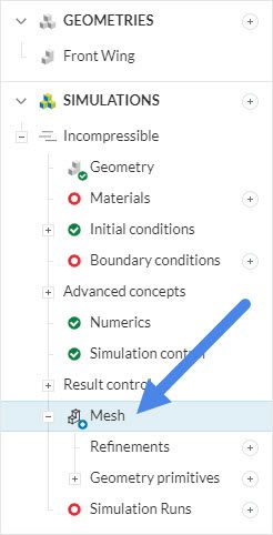
The Hex-dominant parametric mesh does not take into consideration the physics of the simulation while being generated, so it can be set and created before the rest of the simulation settings are applied. Just click on the ‘Mesh’ option in the simulation tree.
- Change the Algorithm to ‘Hex-dominant parametric’.
- Set the cells in the \(\mathrm{X}\) direction to ’20’.
- Set the cells in the \(\mathrm{Y}\) direction to ’10’.
- Set the cells in the \(\mathrm{Z}\) direction to ’10’.
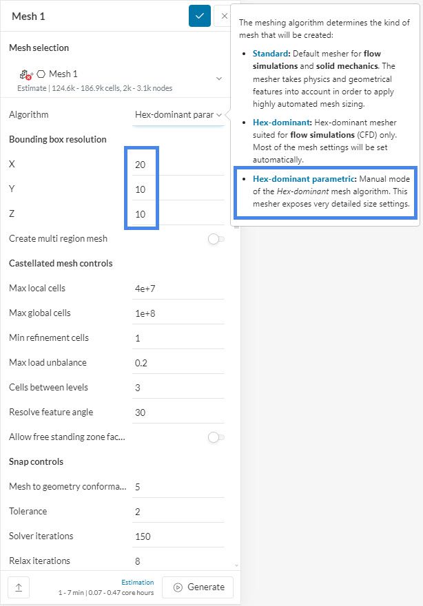
These settings indicate the number of cells that will be created initially at each direction. So, 20 cells will be generated across the \(\mathrm{X}\)-direction, and 10 across the other two. In total, 2000 cells will be generated before any refinements are added.
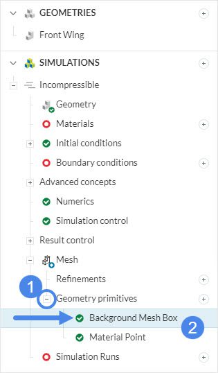
2.1. Background Mesh Box & Material Point
The Background Mesh Box represents the domain of the external simulation and can be accessed from the simulation tree.
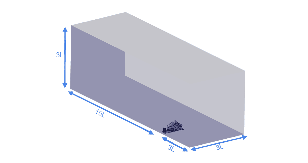
It is recommended that it extends at least 3-5 times the reference length of the object, D, upstream, 8-10 times the D downstream, and 3-5 times the D in the lateral directions. In this tutorial setup, the domain is sized with respect to the length of the wing L in the direction of the wind.
For the creation of the base mesh the user previously specified the number of cells (for the Base Mesh Box) in each coordinate direction under Bounding box resolution.
The base mesh cell size in the \(\mathrm{X}\)-direction for example is then given as:
$$\displaystyle \mathrm{\frac{X_{max} – X_{min}}{N_x}}$$
where \(\mathrm{X_{max}}\) is the maximum \(\mathrm{X}\)-coordinate, \(\mathrm{X_{min}}\) is the minimum \(\mathrm{X}\)-coordinate of the Base Mesh Box and \(\mathrm{N_x}\) is the number of cells in \(\mathrm{X}\)-direction.
Here, the dimensions of the domain, with respect to the chosen sizing seen in Figure 8 is as seen below:
- Minimum x value: ‘-3.73’ \(m\)
- Minimum y value: ‘-2.725’ \(m\)
- Minimum z value: ‘0’ \(m\)
- Maximum x value: ‘5’ \(m\)
- Maximum y value: ‘0’ \(m\)
- Maximum z value: ‘2.725’ \(m\)

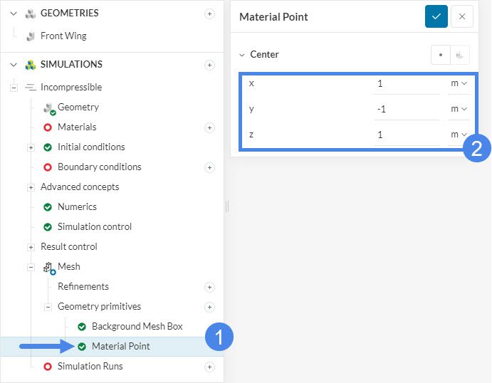
The material point determines whether the resulting mesh is for an External flow simulation or Internal flow simulation. Set its coordinates to ‘(1, -1, 1)’ after clicking on the ‘Material Point’ under the Geometry Primitives item like below:
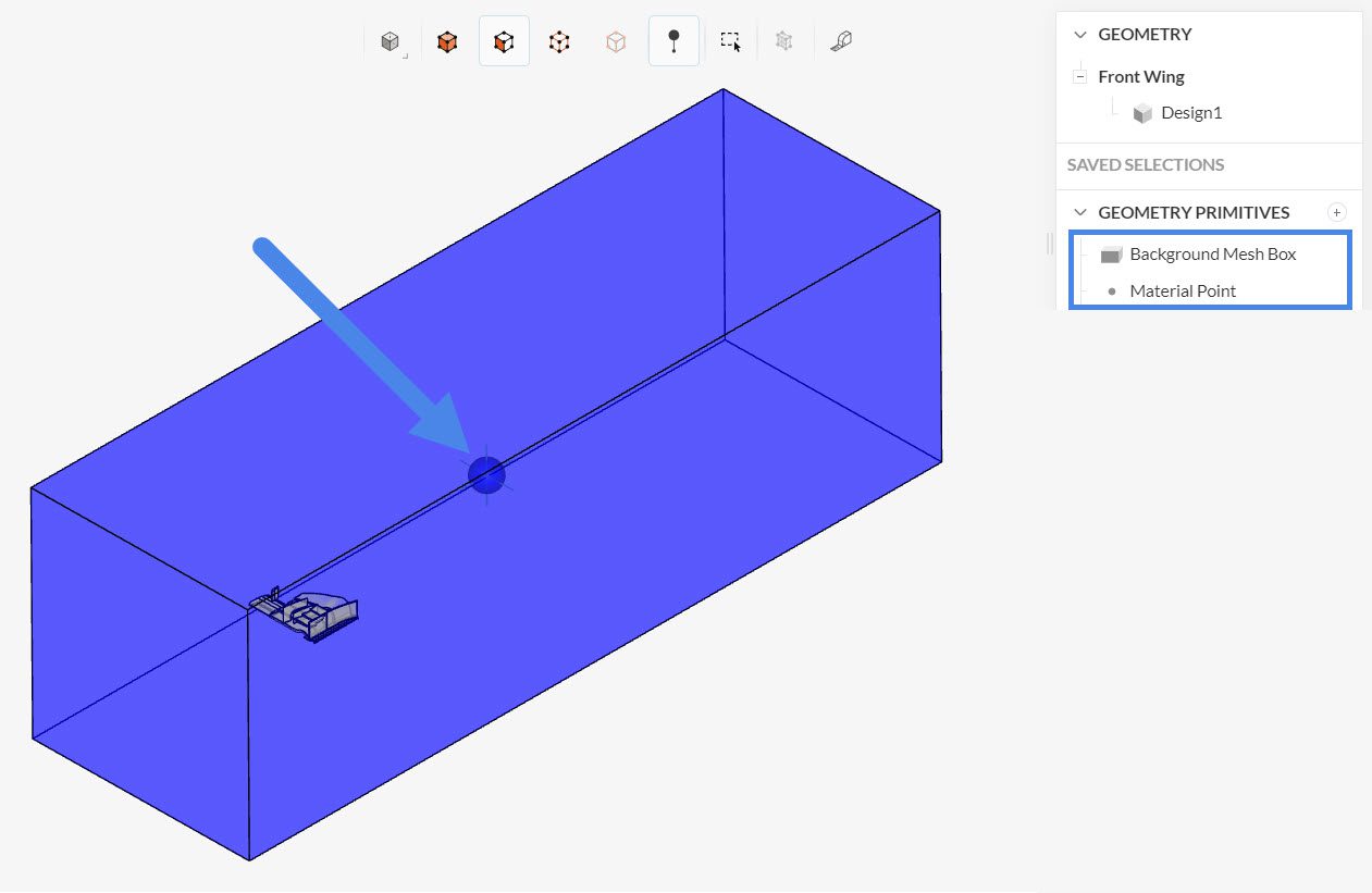
Make sure the point is inside the Background Mesh Box by having them both visible on the geometry tree at the right of the page. It should also not intersect with any face of the model for an external aerodynamic simulation over a watertight geometry.
2.2. Create Geometrical Primitives
Before you add any refinements, create three cartesian boxes and some region refinements will be assigned to each of them afterwards.
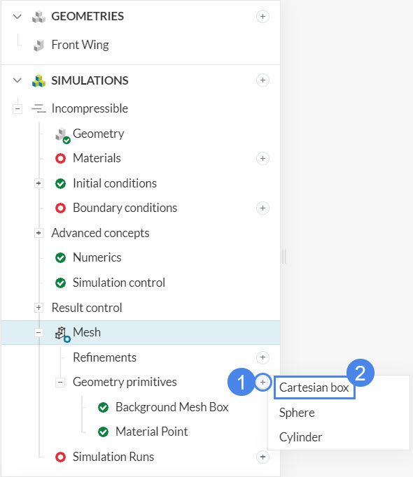
Click on ‘+‘ next to the Geometry primitives, and choose the ‘Cartesian Box’ option like below:
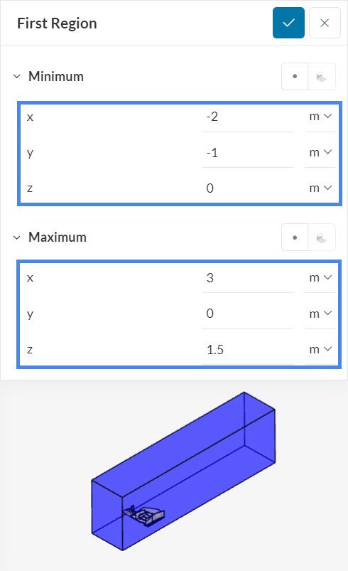
The first cartesian box is the biggest of the three and has the following dimensions, which are set in the same way as the background mesh box, which is by having a maximum and minimum value for each direction:
- Minimum x value: ‘-2’ \(m\)
- Minimum y value: ‘-1’ \(m\)
- Minimum z value: ‘0’ \(m\)
- Maximum x value: ‘3’ \(m\)
- Maximum y value: ‘0’ \(m\)
- Maximum z value: ‘1.5’ \(m\)
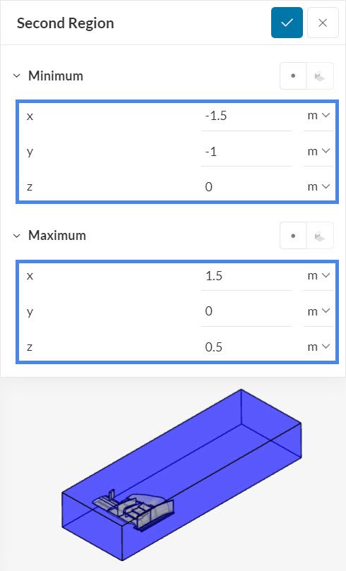
Then create a smaller box, with the following dimensions:
- Minimum x value: ‘-1.5’ \(m\)
- Minimum y value: ‘-1’ \(m\)
- Minimum z value: ‘0’ \(m\)
- Maximum x value: ‘1.5’ \(m\)
- Maximum y value: ‘0’ \(m\)
- Maximum z value: ‘0.5’ \(m\)
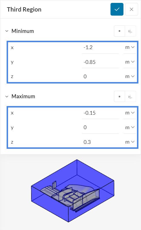
Finally, the smallest box has the dimensions below:
- Minimum x value: ‘-1.2’ \(m\)
- Minimum y value: ‘-0.85’ \(m\)
- Minimum z value: ‘0’ \(m\)
- Maximum x value: ‘-0.15’ \(m\)
- Maximum y value: ‘0’ \(m\)
- Maximum z value: ‘0.3’ \(m\)
2.3. Add Refinements
For the Hex-dominant parametric, several refinement options can be selected by the user to get the required mesh. These are all specified under the Mesh Refinement sub-tree.
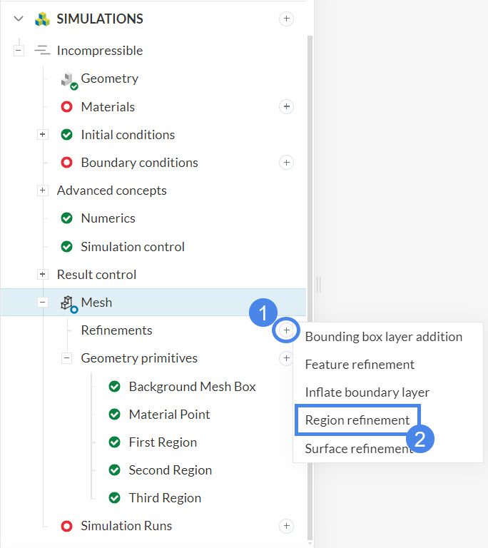
Region Refinements
The region refinement is used to refine the volume mesh for one or more user-specified volume regions under Geometry primitives. Add a Region Refinement by clicking on the ‘+’ icon next to the Refinements, and then choosing the ‘Region Refinement’ option.
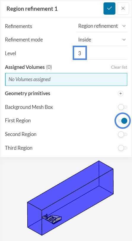
The first region refinement that you will create is matched to the biggest Cartesian box. The Refinement mode will be automatically set to Inside. This refines all volume mesh cells inside the surface up to the specified level. The surface needs to be closed for this to be possible.
- Set the Level to ‘3’
- Toggle on the ‘First Region’ for the assignment.
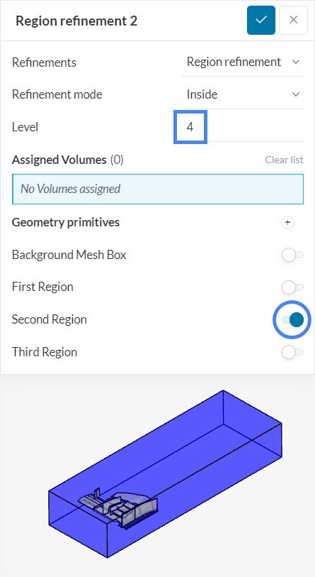
Then add a second region refinement for the medium cartesian box. This time:
- Set the Level to ‘4’.
- Toggle on the ‘Second Region’ for the assignment.
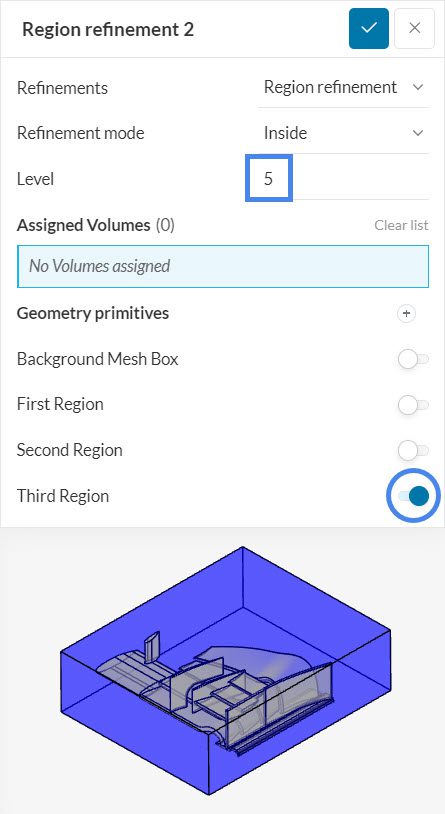
Finally, create a last region refinement for the smallest Cartesian box like before:
- Set the Level to ‘5’.
- Toggle on the ‘Third Region’ for the assignment.
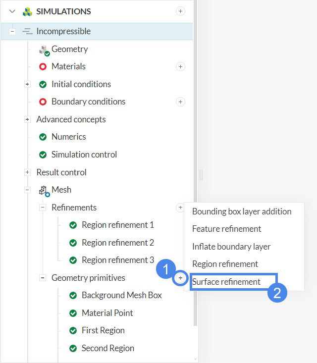
Surface Refinement
Add a surface refinement by clicking on the ‘+’ icon next to the Refinements, and then choosing the ‘Surface Refinement’ option.
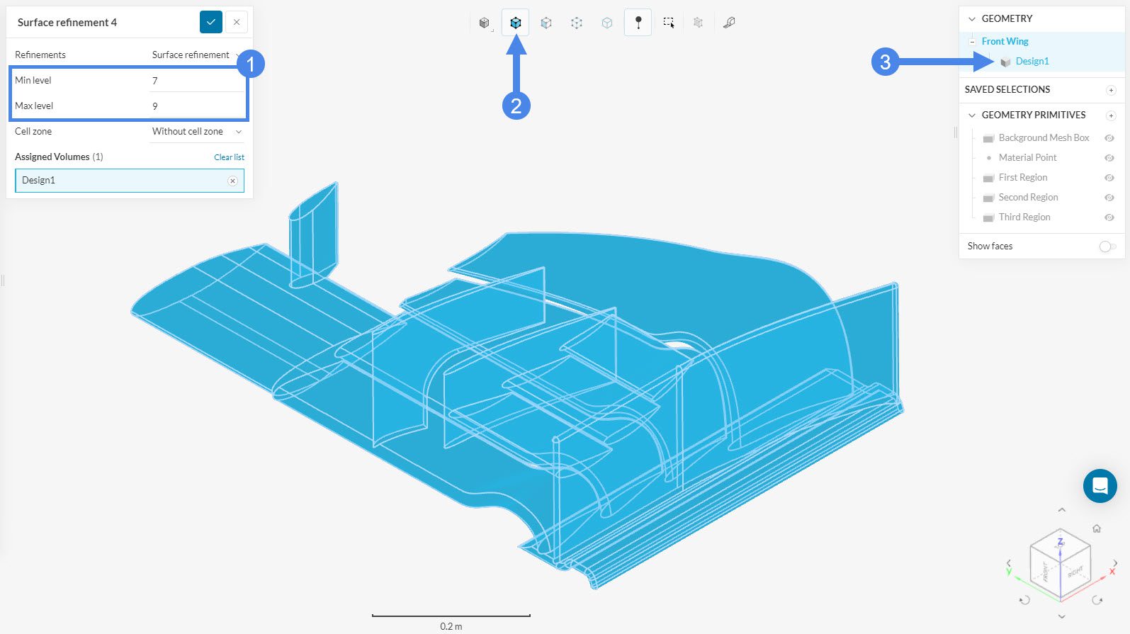
Specify two refinement levels, level min, and level max. The minimum level is applied first across all of the surfaces. The maximum level is only applied to cells in areas where the normals form an angle greater than the specified resolve feature angle (in Advanced Settings).
- Set the minimum refinement level to ‘7’.
- Set the maximum refinement level to ‘9’.
- Toggle on the ‘Assignment’ option.
- Assign the refinement to the whole Front Wing by clicking on ‘Select Volume’ on the top of the page and then on the part on the geometry tree at the right of the page or on the part itself.
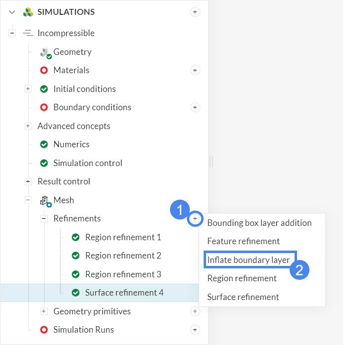
Inflate Boundary Layer
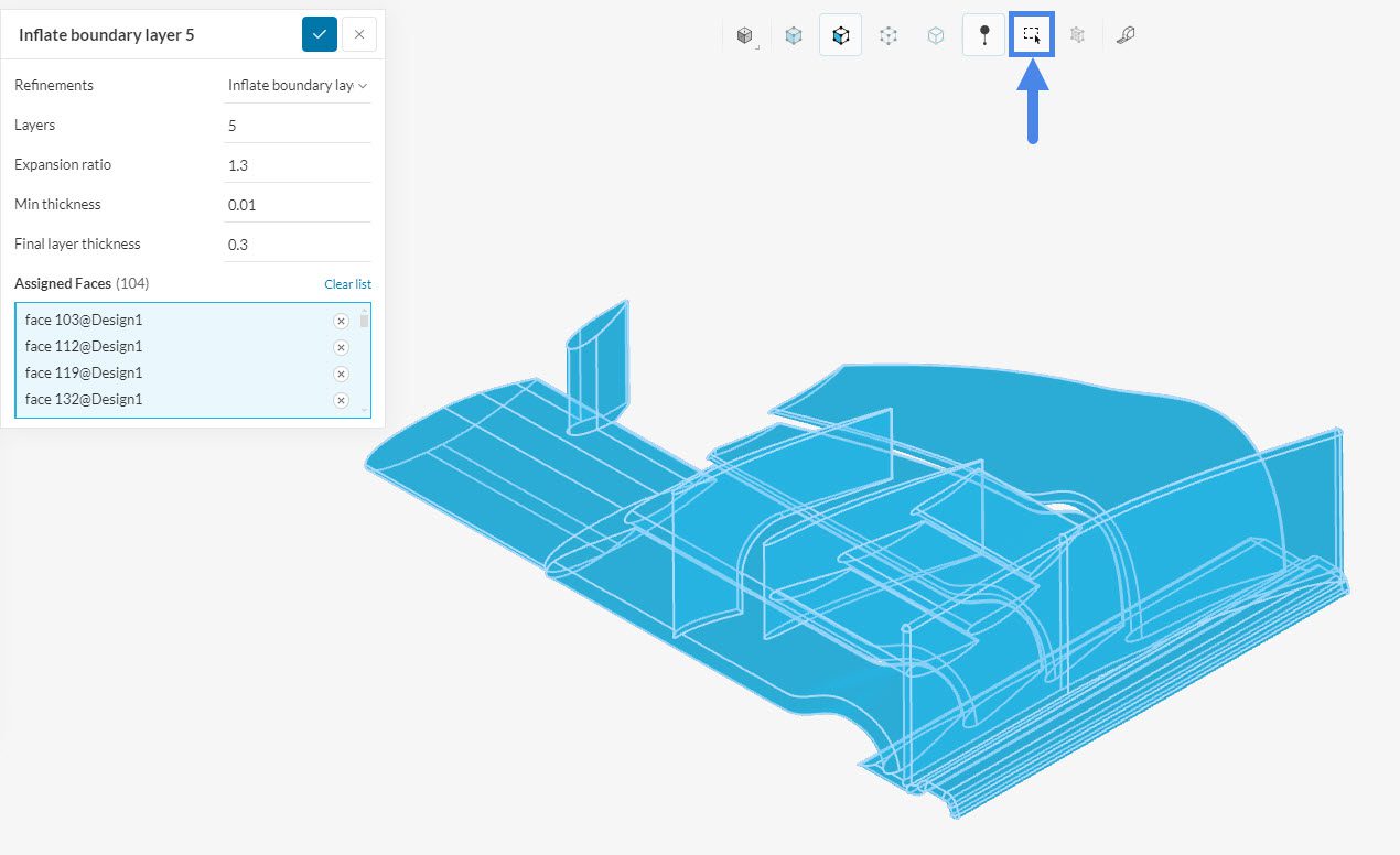
The layer refinement adds a volume mesh with cells aligned to the surface. Add an Inflate boundary layer by clicking on the ‘+’ icon next to the Refinements, and then choosing the ‘Inflate boundary layer’ option.
Leave the values in their default state, and assign this refinement to the front wing by activating the box selection, and then dragging it across the interface holding the left mouse button, so that the whole wing turns light blue. This means that all the faces are selected.
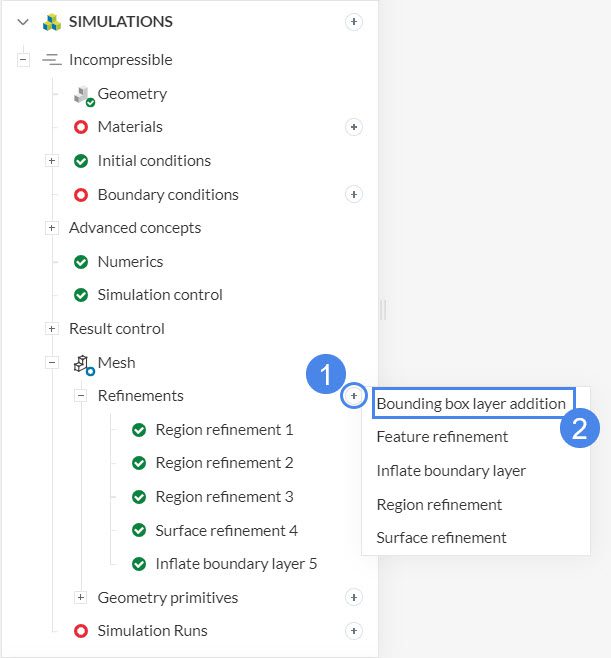
Bounding Box Layer Addition
The Bounding box layer addition refinement is similar to the Layer refinement but only applicable to the bounding box. This is mainly useful for external flow analysis where the box surface acts as a wall for the flow domain and must be refined with a layer mesh for accuracy. Add this by clicking on the ‘+’ icon next to the Refinements, and then choosing the ‘Bounding box layer addition’ option.
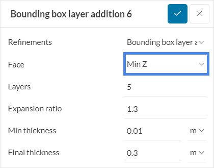
Switch the Face to ‘Min Z’, so that the layers are added to the ground, and keep the rest of the settings at their default state.
Feature Refinement
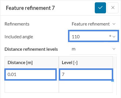
This refinement type is specifically important as it is used to refine the geometry’s feature edges. The feature edges are extracted based on the Included angle. So, the edges whose adjacent surface normals form an angle less than the included angle are marked for extraction and refinement. Click on the ‘+’ icon next to the Refinements, and then choose the ‘Feature refinement’ option.

Change the Included angle to ‘110’ degrees, the Distance to ‘0.01’ and the Level to ‘7’.
The edge and surface mesh will then be refined up until this distance in all directions from the extracted edges.
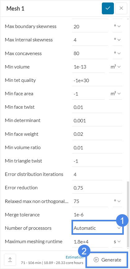
2.4. Generate Mesh
Go back to the Mesh panel, change the Numbers of the processors to ‘Automatic’, for optimal usage of computational power, and click on the ‘Generate’ button in order to start with the mesh creation.
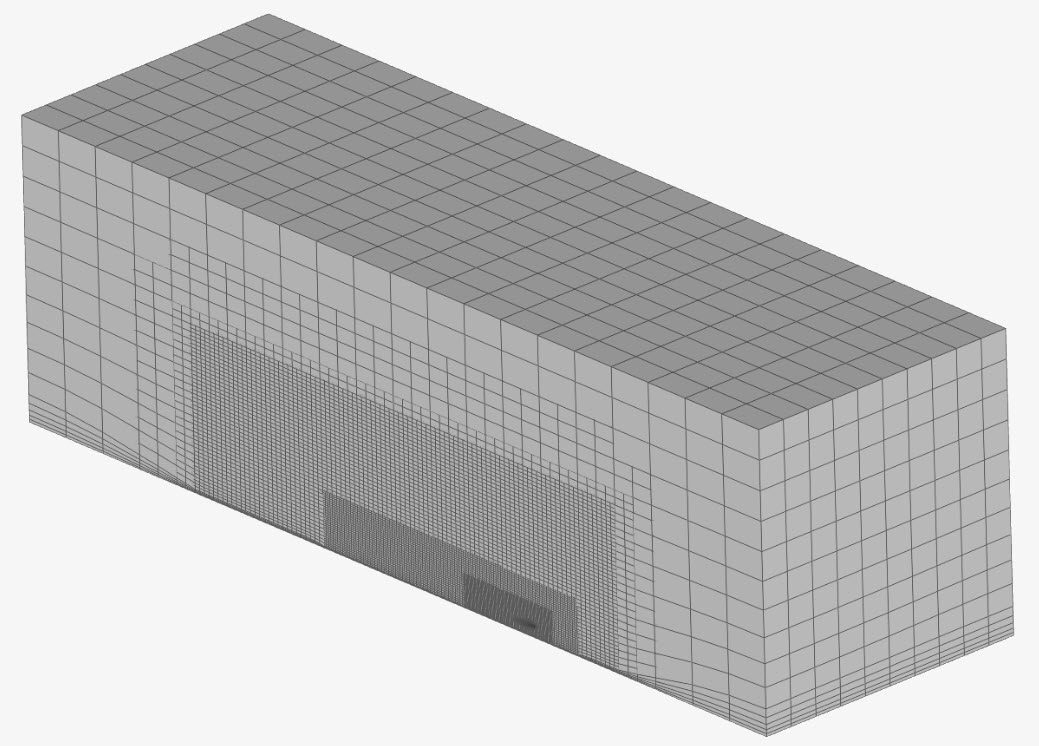
3. Results
After the mesh is ready, the domain will look like this:
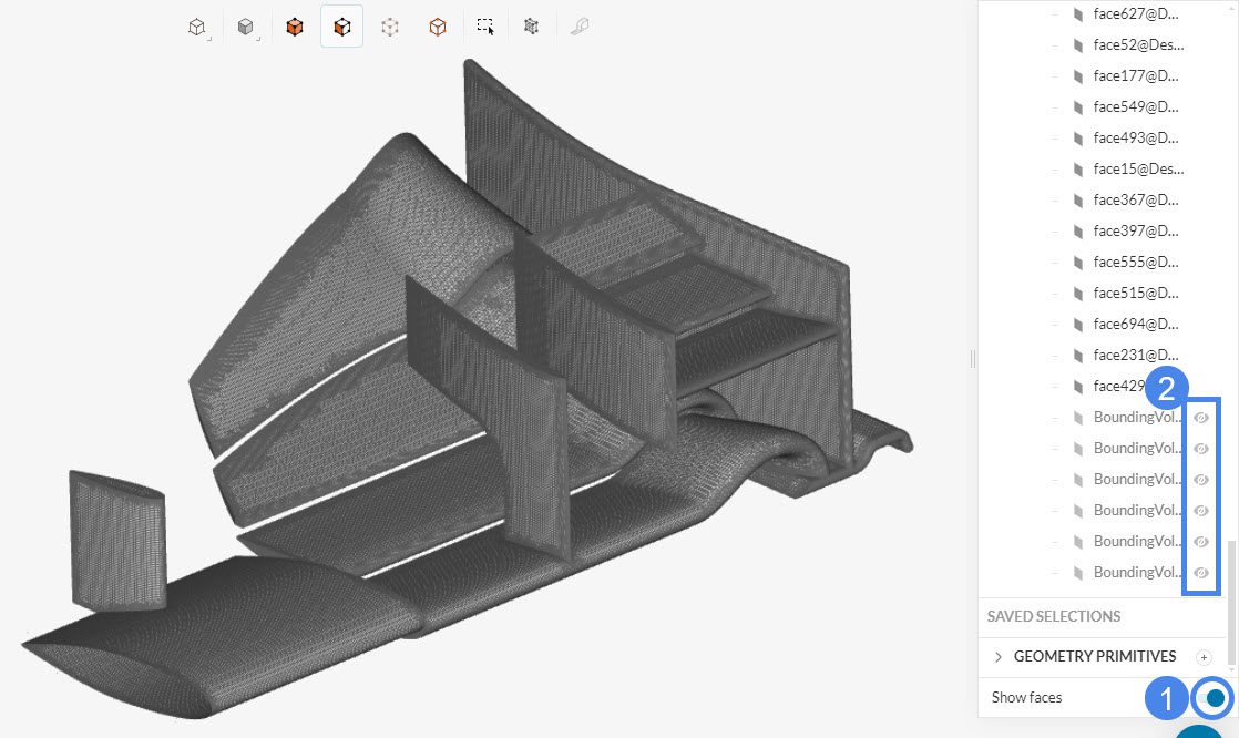
By toggling on the option to Show faces and hiding the faces of the bounding box domain from the tree, you can visualize the final mesh of the front wing:
More details about the mesh can be found under Meshing Log. A quick look at the mesh metrics can be accessed under Event log:
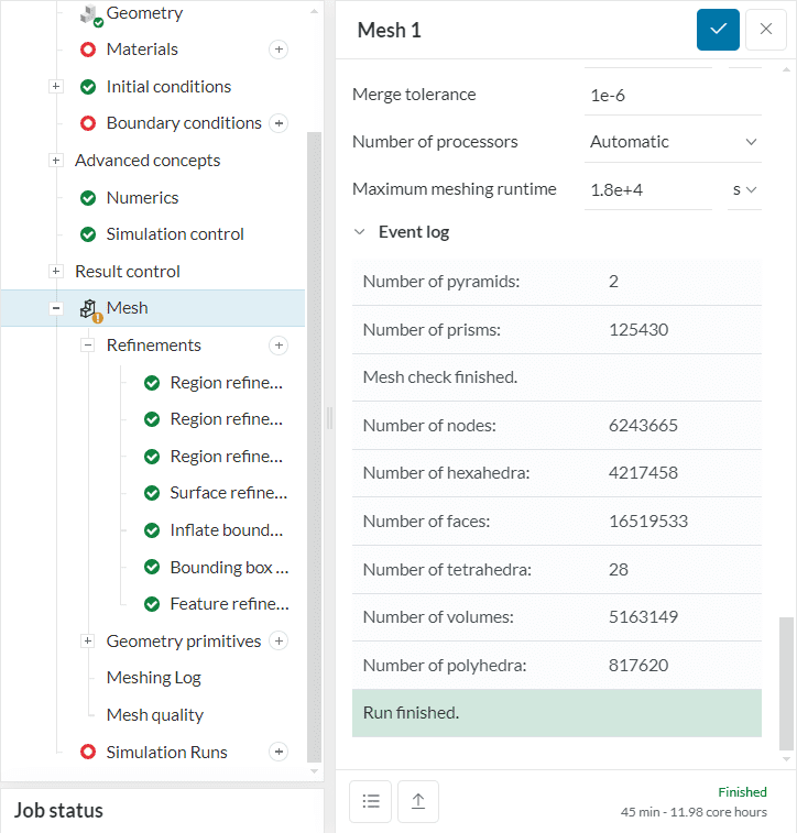
The mesh consists of approximately 4.2 million hexahedral cells, 0.12 million prism cells, 28 tetrahedral cells, and 2 pyramids.
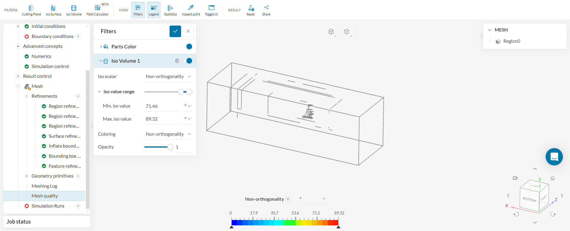
You can check the quality of your mesh and improve it by clicking on the ‘Mesh quality’ in the simulation tree. This will take you to SimScale’s integrated post-processing environment. Use this article to help you visually examine the characteristics of your mesh.
Congratulations! You finished the tutorial!
Note
If you have questions or suggestions, please reach out either via the forum or contact us directly.
Last updated: December 23rd, 2025
Did this article solve your issue?
How can we do better?
We appreciate and value your feedback.


