Validation Case: Turbulent Pipe Flow

This turbulent pipe flow validation case belongs to fluid dynamics. The aim of this test case is to validate the following parameters:

• Pressure drop between the inlet and outlet of the pipe
• Velocity distribution across the flow direction

The simulation results of SimScale were compared to a reference solution based on the Power law velocity profile presented by Henryk Kudela in one of his lectures\(^1\).

Geometry

The geometry can be seen below:

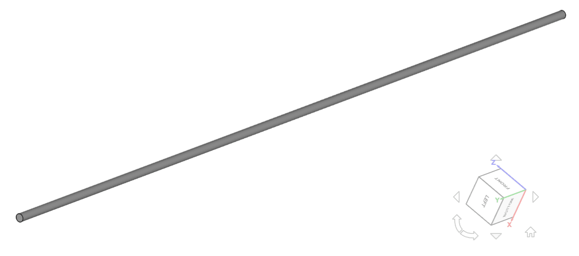
This is a cylindrical pipe with a diameter of 0.01 \(m\), and a length of 1 \(m\).

Analysis Type and Mesh

Tool Type: OpenFOAM®

Analysis Type: Incompressible steady-state analysis.

Turblence Model: Two turbulence models were tested, the k-epsilon and the k-omega SST.

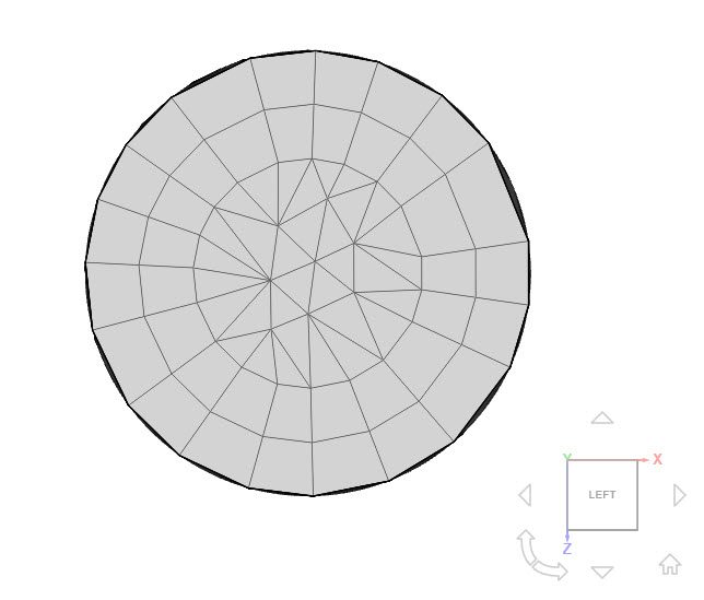
Mesh and Element Types:

Two approaches were tested in this validation case: Wall functions and full resolution on the walls. For the wall functions, the desired \(y^+\) range is [30 , 300], and the generated mesh looks like this:

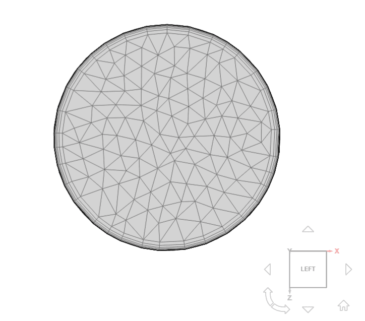
Full resolution on the walls requires a \(y^+\) lower than \(1\), so the final mesh has the following form:

More details about the meshes used in the three cases can be seen bellow:

Cases	Near-wall approach	Number of cells	Mesh type	Turbulence model
A	Wall functions	176574	Standard	k-omega SST
B	Wall functions	176574	Standard	k-epsilon
C	Full resolution	1393776	Standard	k-omega SST

Simulation Setup

Fluid:

• Water
  • \((\nu)\) Kinematic viscosity = 10\(^{-6}\) \(m^2 \over \ s\)
  • \((\rho)\) Density = 1000 \(kg \over\ m^3\)

Boundary Conditions:

• Velocity inlet of 1 \(m \over \ s\)
• Pressure outlet of 0 \(Pa\)
• No-slip walls with wall functions for cases A and B, and full resolution for case C

Initial Conditions:

• Turbulent kinetic energy \((k)\) of 3.84e-3 \(m^2 \over \ s^2\)
• Case A & C: Specific dissipation rate (\(ω\)) of 88.53 \(1 \over \ s\)
• Case B: Dissipation rate \((ε)\) of 3.059e-2 \(m^2 \over \ s^3\)

Reference Solution

The velocity profile for turbulent pipe flow is approximated by the Power-law velocity profile equation \(^1\):

$$\bar{u}_y(r) = \bar{u}_{y_{max}}\left(\frac{R-r}{R}\right)^{1/n}$$

where:

• \({u}_{y_{max}}\): the maximum y-velocity of the cross-section (along the pipe axis)
• \(R\): the radius of the cylinder
• \(r\): the distance from the center of the cross-section
• \(n\): a constant that depends on the Reynolds number, estimated as 7 for this case

For turbulent flow, the ratio of \(u_{y_{max}}\) to the mean flow velocity is a function of \(Re\). In this case, this ratio is calculated to be 1.224.

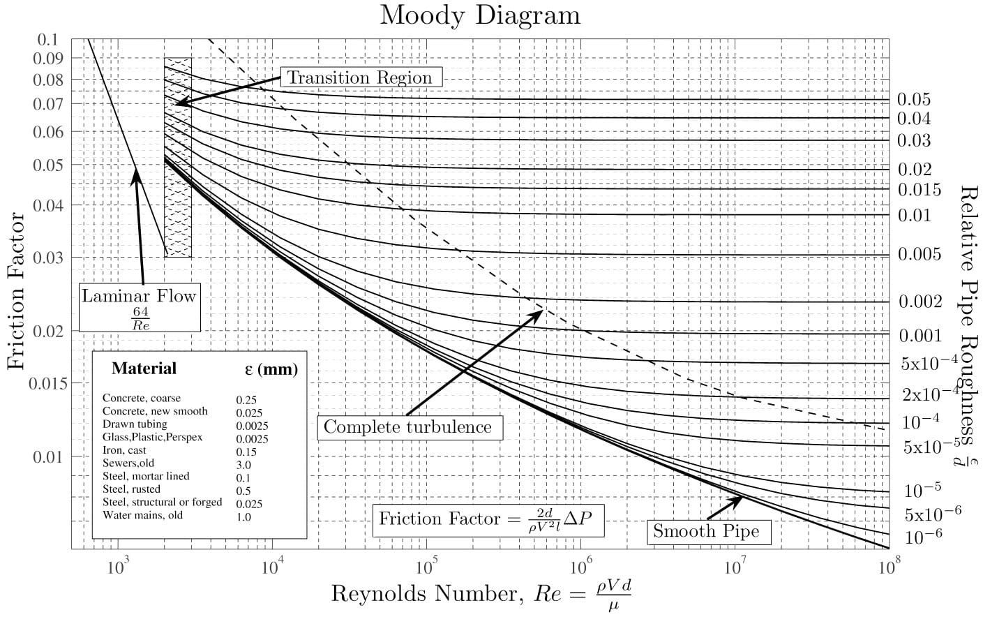
The pressure drop for turbulent flow in pipes is obtained by using the Darcy-Weisbach \(^2\):

$$\Delta P = f\ \frac{\rho\ u^2 \ l}{2 \ d}$$

where:

• \(f\): is the Darcy friction factor calculated by the solution of the Colebrook equation
• \(ρ\): is the density of the fluid
• \(u\): is the average velocity of the cross section
• \(l\): is the length of the pipe
• \(d\): is the diameter of the cylinder

According to the Moody diagram (Figure 4) and for this case, the value of \(f\) is 0.0309.

Result Comparison

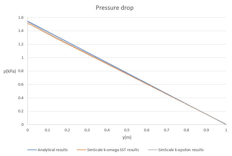
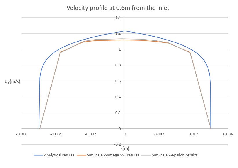
Wall functions

For the “wall function approach” the average \(y^+\) value on the walls of the pipe is 31.95 for k-omega SST and 32.39 for k-epsilon.

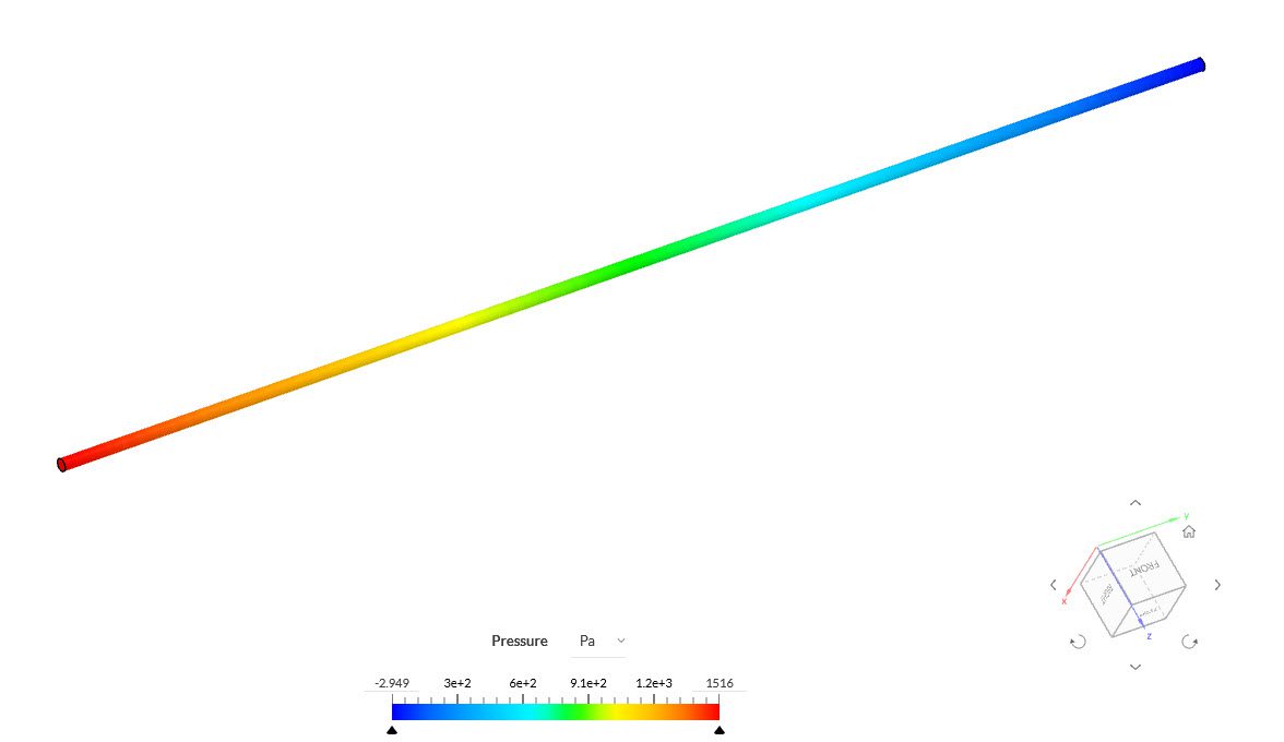
Pressure drop along the pipe length can be observed below:

The following graph shows the developed velocity profile, located 60 \(cm\) from the inlet:

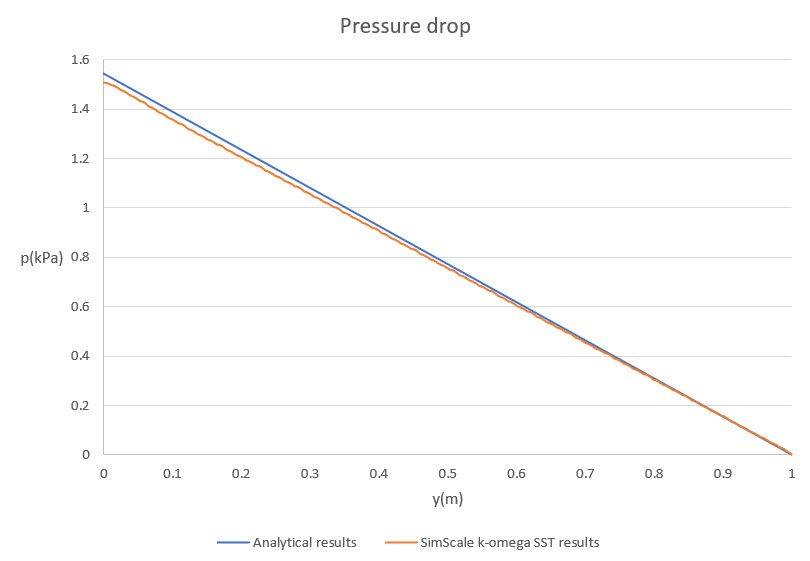
Full resolution

For “full resolution”, the average value for \(y^+\) is 0.017. The corresponding graphs are created:

The pressure drop along the pipe length:

The developed radial velocity profile, located 60 \(cm\) from the inlet:

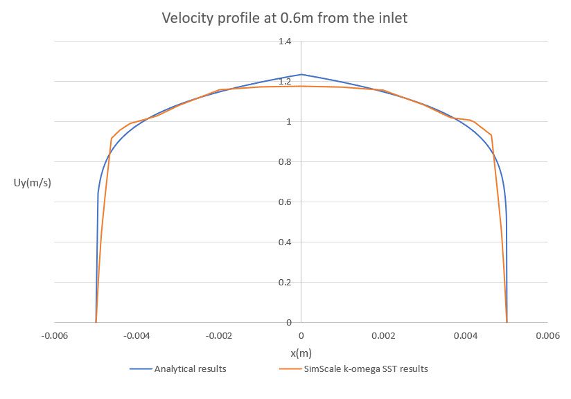
Besides good agreement with the Power law model, results show that all approaches and turbulence models are successful in predicting the pressure drop along pipe length for the given meshes.

Last updated: July 5th, 2023