A mixing tank simulation shows how much power an impeller draws, where the liquid moves slowly or not at all, and how long a feed takes to blend, before the vessel and agitator are bought. Agitator sizing usually starts from correlations measured in a standard tank: four wall baffles, one impeller a third of the tank diameter, and a liquid height equal to the tank diameter. Real vessels add coils, dip pipes, side nozzles, dished bottoms and different liquid levels, and the correlations become less reliable the further the geometry moves from that standard.
Three inputs decide whether a stirred tank model can be trusted: the size of the rotating zone around the impeller, the mesh at the blade tips, and the way power and blend time are measured. Each step below gives a starting value for the input and a way to check it.
How to set up a mixing tank simulation in 8 steps
Model only the liquid, put the impeller inside a rotating zone, and solve a steady-state incompressible flow with the multiple reference frame (MRF) method. Check the impeller power number against its published value before you read the flow pattern, then run a transient case with a tracer to measure blend time. The eight steps below build that model in order in SimScale. Step 8 covers tanks where the free surface or a second liquid changes the result.
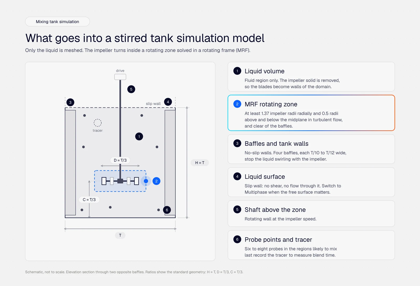
The examples use one tank throughout: 1.2 m diameter, filled with water to 1.2 m, four baffles 0.12 m wide, and a 0.4 m impeller 0.4 m off the bottom, turning at 120 rpm.
Step 1: Calculate the impeller Reynolds number
Calculate the impeller Reynolds number from the rotational speed, the impeller diameter and the fluid properties. It decides the turbulence model in step 4 and which design correlations you can check the result against.
$$ \mathrm{Re} = \frac{\rho N D^2}{\mu} $$
Here ρ is the liquid density, N is the rotational speed in revolutions per second, D is the impeller diameter (not the tank diameter) and μ is the dynamic viscosity.
| Impeller Reynolds number | Regime | What changes |
|---|---|---|
| Below about 10 | Laminar | Power number falls in proportion to 1/Re. Baffles have little effect. |
| About 10 to 10,000 | Transitional | Power number and flow pattern still change with Re. |
| Above about 10,000 | Fully turbulent | Power number is constant for a given impeller and tank geometry. |
For the example tank, water at 20 °C (ρ = 998 kg/m³, μ = 0.001 Pa·s) with D = 0.4 m and N = 2 rev/s gives Re ≈ 3.2 × 10⁵, well inside the turbulent range. The impeller tip speed, πND, is 2.5 m/s.
For a shear-thinning or yield-stress liquid, assign a non-Newtonian viscosity model such as power law or Herschel-Bulkley. Viscosity then varies with the local shear rate, so the Reynolds number above is only an estimate.
Step 2: Prepare the tank geometry and the liquid volume
Extract the liquid volume from the vessel CAD, keep every internal that sits in the flow path, and remove the impeller solid so that the blades become walls of the fluid region.
- Keep: baffles, impeller blades and hub at their real thickness, the shaft, the bottom head shape, and any coils, dip pipes, spargers and nozzles below the liquid level.
- Remove: the motor, gearbox, mounting brackets, flange bolts and anything outside the wetted volume.
- Liquid surface: for a baffled tank, cut the liquid volume at the liquid level. That flat face becomes a slip wall in step 4. Model the headspace only when you need the free surface itself (step 8).
- Fluid region: extract the liquid region from the vessel CAD with flow volume extraction in SimScale, or build it in your own CAD tool, trimmed at the liquid level.
Most published power numbers and mixing tank design correlations were measured in one standard geometry. Compare your vessel against it before you start:
| Ratio | Standard value | Example tank |
|---|---|---|
| Liquid height to tank diameter, H/T | 1 | 1.2 m / 1.2 m |
| Impeller diameter to tank diameter, D/T | 1/3 | 0.4 m |
| Impeller clearance off the bottom, C/T | 1/3 | 0.4 m |
| Baffles | 4, each T/10 to T/12 wide | 4 × 0.12 m (T/10) |
The further your vessel departs from these ratios, the less a textbook power number or blend time applies to it.
Step 3: Create the rotating zone around the impeller
Add a cylindrical volume that encloses the impeller and hub, shares the shaft axis, and stays clear of the baffles. This volume becomes the MRF rotating zone.
SimScale’s guide to preparing CAD for rotating zones sets the structure: one fluid volume plus one overlapping volume per rotating zone, with the impeller solid removed. The From faces cylinder in CAD Edit builds the zone around the selected blade faces. A clearance factor of 1.1, the value recommended for rotating machinery, suits a pump impeller in a close-fitting casing. A stirred tank has more room between the blade tips and the baffles, and the zone should use it.
- Zone size: in one MRF study of a baffled tank with a high-shear impeller (Santos-Violante et al., AIChE Annual Meeting 2020), turbulent velocity profiles agreed once the zone reached 1.367 impeller radii in the radial direction and 0.505 impeller radii above and below the impeller midplane. Smaller zones showed significant discrepancies. In laminar flow, the zone size made no relevant difference.
- Example tank: a zone radius of at least 0.27 m (1.37 × 0.2 m) still leaves 0.21 m to the baffle edges at 0.48 m. Extend the zone at least 0.1 m above and below the impeller midplane, and further if the blades reach beyond that.
- Clearance: keep every face of the zone away from the blade edges. A zone face that is tangential to a blade causes an incorrect rotating zone error.
- Axis and direction: set the rotation axis along the shaft. SimScale uses the right-hand rule, with the thumb along the axis. For a pitched blade turbine or hydrofoil, check the direction against the pumping direction you want: reversing the rotation turns a down-pumping impeller into an up-pumping one.
Full setup details are on the rotating zones documentation page.
Step 4: Set up the analysis, materials and boundary conditions
For a single liquid in turbulent flow, use the Incompressible analysis type, steady state, with an MRF rotating zone and the k-omega SST turbulence model.
- Rotating zone: MRF, at the impeller speed (120 rpm in the example). MRF solves the zone in a rotating frame at one blade position relative to the baffles, without moving the mesh, which makes it much cheaper than a transient rotating mesh.
- Turbulence model: k-omega SST is a practical default above Re ≈ 10,000. Standard k-epsilon is the model used in many published stirred tank comparisons. Below Re ≈ 10, set the flow to laminar.
- Material: density and viscosity at the process temperature, with a non-Newtonian model where step 1 called for one.
Assign the boundary conditions by surface:
| Surface | Boundary condition |
|---|---|
| Tank wall, bottom and baffles | No-slip wall (the default for unassigned faces) |
| Impeller blades and hub inside the zone | None needed: walls inside the MRF zone rotate with it |
| Shaft outside the zone | Rotating wall, at the impeller speed about the shaft axis |
| Stationary surfaces inside the zone, such as a dip pipe | Rotating wall with zero rotational velocity |
| Liquid surface | Slip wall: no shear, no flow through the surface |
| Feed and outlet nozzles (continuous tanks only) | Velocity inlet and pressure outlet |
The wall boundary condition page covers the slip and rotating wall options.
Step 5: Mesh the impeller region
Use the standard mesher with physics-based meshing, refine the rotating zone and the blade surfaces, and confirm that the power number stops changing with refinement.
- Cell zone: with physics-based meshing enabled, the mesher creates the cell zone for the rotating zone automatically. Without it, define the cell zone manually.
- Region refinement: make cells inside the rotating zone finer than in the bulk of the tank. The stream leaving the blade tips carries the steepest velocity gradients and most of the turbulence.
- Surface refinement: refine the blades, the disc of a Rushton turbine, and the baffle edges, where the flow separates.
- Inflation layers: add a few layers on the blades and baffles so the wall treatment of the turbulence model has cells to work with.
- Convergence check: run the case on a coarse and a refined mesh. If the power number from step 6 moves by more than about 5%, refine again.
Step 6: Solve the steady case and check the power number
Add a forces and moments result control on the impeller and shaft, convert the torque to power, and compare the resulting power number with the published value for your impeller before you read the flow pattern.
The forces and moments result control integrates pressure and skin friction over the selected surfaces. Select the blades, hub, disc and shaft, and place the center of rotation on the shaft axis. The moment component about the axis is the impeller torque, M. Then:
$$ P = 2 \pi N M $$
$$ N_p = \frac{P}{\rho N^3 D^5} $$
| Impeller | Flow pattern | Turbulent power number, Np | Typical duty |
|---|---|---|---|
| Rushton turbine (6-blade disc) | Radial | About 5 | Gas dispersion, high shear |
| Pitched blade turbine (4 blades, 45°) | Mixed, mostly axial | About 1.3 | Blending, solids suspension |
| Hydrofoil | Axial | About 0.3 | Blending and suspension at low power |
Values are for fully turbulent flow in a standard baffled tank and shift with blade thickness, D/T and C/T. Use the impeller manufacturer’s value where you have it.
For the example tank with a Rushton turbine, Np ≈ 5 gives P ≈ 410 W and a torque of about 32.5 N·m at 120 rpm. If the simulated power number is within about 10% of the published value, the rotating zone and mesh are adequate to read the flow. If it is not, check the zone size and the mesh at the blade tips first.
Calculate power from torque, not from the volume integral of turbulent dissipation, which RANS models under-predict near the impeller. In a published Rushton turbine comparison at Re = 29,000 (Gimbun et al., AIChE Journal, 2012), standard k-epsilon with an MRF zone gave a power number of 4.72 from torque against 4.99 measured, but 3.99 from the dissipation integral.
Judge convergence on the torque as well as the residuals. If the torque keeps oscillating instead of settling, the flow in the zone has large transient features, often because the blades pass close to baffles or internals. Use an arbitrary mesh interface (AMI) rotating zone in a transient run for that case.
Step 7: Measure blend time with a tracer
Run a transient case with a passive scalar released at the feed point, track it with probe points, and take the blend time as the moment every probe stays within 5% of the final concentration.
- Analysis: Incompressible, transient. Keep the MRF zone if the steady case showed no large transient features in it. Otherwise use an AMI zone, with a time step that turns the impeller about 1 to 2 degrees per step (2.8 ms for 2 degrees at 120 rpm).
- Tracer: enable passive scalar transport in the global settings. In the initial conditions, set the scalar to 1 inside a small subdomain at the feed location and 0 everywhere else. The fully mixed value is then the subdomain volume divided by the liquid volume, so you know the target before the run.
- Probes: place six to eight probe points, including the regions likely to mix last: below the impeller near the bottom, behind a baffle, and just under the liquid surface.
- Time step and end time: use an adjustable time step with a maximum Courant number of about 1, and an end time several times the correlation estimate below.
The transient run starts from rest, so the measured time includes the flow spinning up. Use it to compare design variants run with the same setup, and check the absolute value against the Grenville and Nienow correlation for turbulent blending in a baffled tank (Handbook of Industrial Mixing, 2004):
$$ \theta_{95} = \frac{5.20 \, T^{1.5} H^{0.5}}{N D^2 N_p^{1/3}} $$
For \( H = T \), this reduces to \( \theta_{95} = \frac{5.20}{N N_p^{1/3}} \left( \frac{T}{D} \right)^2 \), which gives about 14 s for the example tank with a Rushton turbine at 120 rpm. A hydrofoil at the same speed gives about 35 s, at about 6% of the power. Rearranged, the correlation gives the same blend time for any impeller type at the same power draw and diameter: the hydrofoil reaches 14 s at about 307 rpm. For blending alone, the impeller choice then comes down to shaft speed, torque and the tank’s other duties, such as solids suspension or gas dispersion.
For a continuous-flow tank, add the mean age of fluid field calculation to the steady case. It shows how long the liquid has been in the tank at every point, which exposes short-circuiting and the regions where liquid stays longest.
Step 8: Add the free surface or a second liquid
Switch to the Multiphase analysis type when the surface vortex, air entrainment or a second immiscible liquid affects the result. It tracks two immiscible fluids with the volume of fluid (VOF) method and always runs transient.
Typical cases are unbaffled tanks with a central vortex, low liquid levels or impellers close to the surface, and two immiscible liquids such as oil and water. The setup changes from steps 2 to 7 are:
- Domain: include the headspace above the liquid, closed at the vessel top.
- Materials: assign both fluids to the same volume, then initialize the phase fraction with a subdomain below the liquid level. Use 0 or 1 only, never intermediate values. Multiphase materials assignment and initialization walks through it.
- Rotating zone: available in the Multiphase analysis only with local time stepping disabled.
- Mesh: use the hex-dominant (parametric) mesher with uniform cells, at most one boundary layer, and thin baffles and blades thickened so the cells can stay coarser. Smaller cells force smaller time steps. See best practices on meshing a multiphase flow analysis.
- Time step: adjustable, with a maximum Courant number and maximum alpha Courant number of 0.7 as a starting point. Why multiphase simulations take so long explains the trade-off.
- Tip speed: keep πND within the 15 m/s flow speed documented for the Multiphase analysis.
- Monitoring: place probe points to record phase fraction over time. When the readings stop changing, the phase distribution has stabilized.
VOF resolves interfaces that span several cells, and droplets smaller than the local cell size are not tracked individually. For a liquid-liquid tank, read the phase fraction distribution rather than a droplet size. The Multi-purpose analysis type also runs VOF multiphase, and SPH simulation is the mesh-free alternative for flows dominated by splashing.
How to check mixing tank simulation results
Read the velocity plots only after the model passes four checks. Each one catches a setup error that still produces a plausible-looking flow pattern.
- Power number: within about 10% of the published or measured value for your impeller (step 6).
- Rotating zone size: enlarge the zone radius by about 20% and re-run. If the power number moves by more than a few percent, the original zone was too small.
- Mesh: the power number moves by less than about 5% on a refined mesh (step 5).
- Convergence: the torque and the velocity at a few probe points are flat over the last iterations, and the residuals have dropped and leveled off.
Then read the flow. Plot velocity magnitude on a vertical plane through a baffle, one midway between two baffles, and horizontal planes at several heights, with the same color scale for every design variant. The usual low-velocity regions are the bottom corners, the space below the impeller, the wake behind each baffle, and the upper liquid in tall tanks.
To fix a slow region, lower the impeller to sweep the bottom, change to an axial impeller for top-to-bottom circulation, add a second impeller on the shaft of a tall tank, or change the speed. Re-run the same setup and compare power number, blend time and the low-velocity regions side by side. Rotating zone speed can be varied in a parametric study, so a speed sweep runs from one setup.
Jet-mixed and flow-through tanks
Tanks mixed by nozzles, or only by the flow passing through them, use the same workflow without a rotating zone. Model the nozzles as velocity inlets and the suction or outlet as an outlet, then judge mixing from the velocity field and the mean age of fluid.
- Aquabio simulated a 27.3 m diameter anaerobic reactor tank mixed by two banks of six angled nozzles, with a total flow of 1,600 m³/h. The team checked mixing at the 9 m and 11.5 m liquid levels, and found the tank still mixed sufficiently with one of its two pumps switched off. At full capacity, the top 1.5 m of liquid mixed at a reduced rate.
- JESA ran steady-state incompressible simulations of baffle layouts for a triangular buffer tank in a wastewater plant. The best layout avoided short-circuiting, reduced dead zones by 30% against the baseline, and cut the mean water age from 24 hours to 11 hours.
- Allegro Energy designs electrolyte tanks of 15,000 to more than 100,000 liters for its flow batteries. The team runs two-phase simulations of the electrolyte with the tank’s nitrogen headspace in the Multi-purpose analysis, and liquid-only incompressible runs to calculate residence time. A typical tank takes 10 to 30 simulations of baffle designs, flow rate and nozzle shape, depth and orientation before it goes to a fabricator.

Finn Trass
Process Flow Engineer, Allegro Energy

“If the tank isn’t well mixed, you might turn an 8-hour battery into a 4-hour battery, because half of your electrolyte isn’t being used. Simulation is the only way to really assess how well the tank performs.”
Run a mixing tank simulation with Engineering AI
SimScale’s Engineering AI agent can build a multiphase mixing tank setup from the CAD and a single request.
In a SimScale demo, the agent set up an oil and water mixing simulation in a stirred tank. Working from the CAD alone, it checked the center of gravity of each part to find where the fluid region needed to be, built the rotating region around the impeller, and removed the solids not needed for the simulation. It then assigned water and oil as separate phases and placed eight probe points through the tank to track phase fraction over time. When those readings flatten out, the mixture has stabilized.
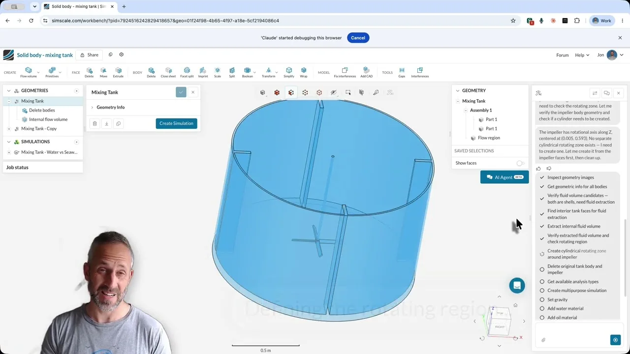
Use steps 1 to 8 as a review checklist for the agent’s setup. Check the rotating zone size, the rotation speed and direction, the phase initialization and the probe positions before you read the results. Engineering AI, explained covers how the agent works across other analysis types.
Mixing tank simulation examples to copy
These public projects, tutorials and validation cases cover the parts of the setup above. Copy a project into your workspace to start from a working model.
- Stirred tank reactor with multiphase flow: a stirred tank reactor with a propeller impeller, run with the Multiphase analysis.
- Tank agitation: an open-top tank with an agitator, run as eight Incompressible cases that vary blade count, blade angle, impeller type and rotational speed.
- Pharmaceutical liquid-liquid mixing: transient Incompressible mixing runs, linked from the pharmaceutical mixing application page.
- Drone simulation using rotating zones: a step-by-step tutorial for an MRF rotating zone.
- Fluid flow simulation through a centrifugal pump: an advanced tutorial with a steady-state MRF zone around an impeller.
- Scalar transport in a T-junction pipe: a validation case for passive scalar mixing against experimental data.
- 3D dam break: a validation case for the Multi-purpose VOF solver against experimental data from Kleefsman et al.
For the full range of mixing capabilities, see multiphase flow simulation, pharmaceutical mixing and impeller design.
Run your first mixing tank simulation in the browser
Set up the rotating zone, mesh and tracer yourself, or let Engineering AI build the setup for you.
Frequently asked questions
A mixing tank simulation is a CFD model of the liquid in a stirred or jet-mixed vessel. It predicts the velocity field, stagnant regions, impeller power and torque, and blend time. With a multiphase model, it also predicts the free surface and the distribution of a second phase.
The impeller sits inside a rotating zone. The multiple reference frame (MRF) method solves the zone in a rotating frame at one impeller position, which is steady-state and fast. The arbitrary mesh interface (AMI), or sliding mesh, method rotates the zone’s mesh every time step, which is transient and slower but resolves the interaction between blades and baffles.
Above an impeller Reynolds number of about 10,000, k-omega SST is a practical default, and standard k-epsilon is used in many published stirred tank studies. Below about 10, the flow is laminar and needs no turbulence model. With either RANS model, calculate power from impeller torque rather than from the integral of turbulent dissipation, which RANS models under-predict.
Power is P = Np ρ N³ D⁵, where Np is the impeller power number, ρ the liquid density, N the speed in revolutions per second and D the impeller diameter. In a fully turbulent baffled tank, Np is about 5 for a Rushton turbine, 1.3 for a 45° pitched blade turbine and 0.3 for a hydrofoil. From a simulation, P = 2πNM, where M is the impeller torque.
For turbulent blending in a baffled tank with the liquid height equal to the tank diameter, the Grenville and Nienow correlation gives θ95 = 5.20 (T/D)² / (N ∛Np), the time to reach 95% uniformity. In a simulation, release a passive scalar tracer at the feed point and record it at probe points until every probe stays within 5% of the final concentration.
The standard geometry has a liquid height equal to the tank diameter (H/T = 1), an impeller diameter and bottom clearance of one third of the tank diameter (D/T = C/T = 1/3), and four wall baffles each T/10 to T/12 wide. Most published power numbers and blend time correlations were measured in this geometry.
Tanks with low-viscosity liquids in turbulent flow do. Without baffles, the liquid rotates with the impeller, a central vortex forms, the power draw falls and top-to-bottom circulation weakens. In laminar mixing of very viscous liquids, baffles have little effect.
You need one when the free surface, air entrainment or a second immiscible liquid affects the result. Typical cases are unbaffled tanks with a deep vortex, low liquid levels, impellers close to the surface, and liquid-liquid systems such as oil and water. SimScale’s Multiphase analysis uses the volume of fluid (VOF) method and always runs transient.
Start from a working setup
The quickest way to a first result is to copy a public mixing project or the rotating zones tutorial, swap in your vessel and impeller, and run the steady MRF case. Once the power number matches the published value for your impeller, run the tracer case for blend time and compare design variants with the same setup.