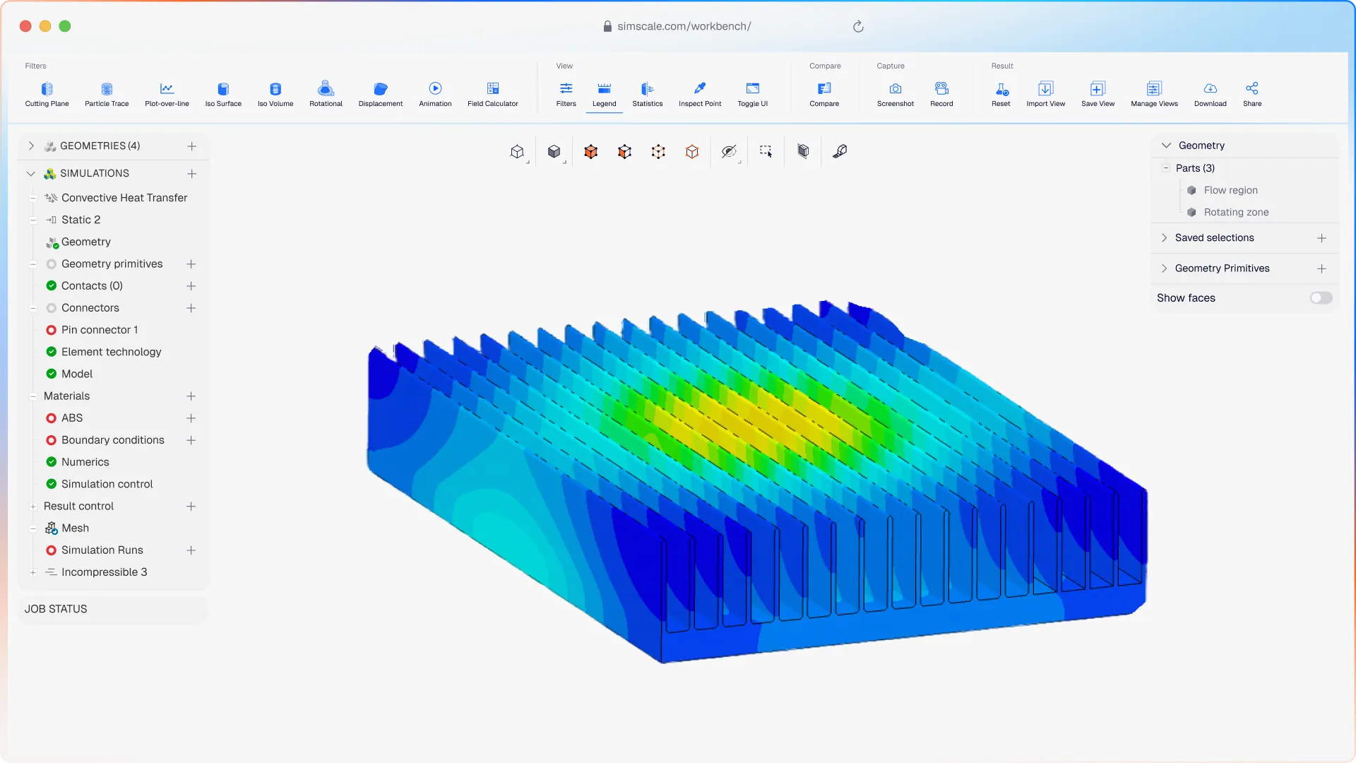

The bench measurement rarely matches the datasheet. You size a heat sink to 2.1 °C/W, order the extrusion, build the board, and the junction runs 12 °C hotter than the calculation predicted. At that point the design has to be reworked quickly to avoid disrupting the schedule.
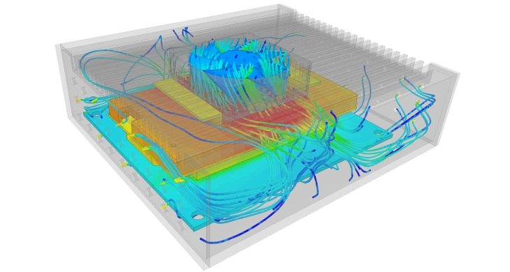
The difference comes from testing conditions. A heat sink measured on its own in a wind tunnel behaves differently from the same heat sink installed in your enclosure, next to other heat sources, with a share of the air passing around the fin array rather than through it. Predicting that is where simulation helps: it gives component temperatures in the real assembly under the real boundary conditions, and it lets you compare many heat sink designs to find the one that meets your requirements.
This guide covers the sizing calculation to do before touching CAD, the geometry variables worth varying, and how to run 50 fin geometries as a single batch.
How do I calculate the required thermal resistance of a heat sink?
Subtract the resistances you cannot change from the total your temperature budget allows:
$$ \theta_{sa} = \frac{T_{j,max} – T_a}{P_D} – \theta_{jc} – \theta_{cs} $$
Where \(\theta_{sa}\) is the highest sink-to-ambient resistance the design can tolerate, \(\theta_{jc}\) is junction-to-case from the component datasheet, and \(\theta_{cs}\) is case-to-sink, set by the thermal interface material.
A worked example. A MOSFET dissipates 25 W. The datasheet rates \(T_{j,max}\) at 150 °C, and you derate to 125 °C for margin. Worst-case ambient inside the enclosure is 45 °C. \(\theta_{jc}\) is 0.8 °C/W and the interface pad contributes 0.3 °C/W.
\(\theta_{sa}\) = (125 − 45) / 25 − 0.8 − 0.3 = 3.2 − 1.1 = 2.1 °C/W

This result determines the rest of the design. It indicates whether a stamped clip-on heat sink is sufficient, whether an extrusion with 40 mm fins is needed, or whether the only way to achieve the required cooling is to add a fan to increase heat transfer. Calculate it first, and use the ambient temperature the product will see in service rather than 25 °C.
Two inputs are commonly underestimated. The first is the junction temperature limit: designing to the absolute rating leaves no allowance for component aging, manufacturing tolerance, or a unit installed in an unusually hot environment, so derate \(T_{j,max}\). The second is dissipated power: use the real \(P_D\), including switching losses at the highest duty cycle the firmware permits, rather than the steady-state figure.
For more detail on the underlying concept, see our separate article on what thermal resistance really measures.
The limits of the hand calculation
The \(\theta_{sa}\) equation assumes a heat sink in clean, fully developed flow with heat entering the base uniformly. A real board meets none of those conditions, and four effects account for most of the resulting error.
Spreading resistance. A 6 mm die on a 60 mm base does not heat the base uniformly. Heat concentrates near the source, the outer fins run cooler than average, and the effective resistance rises. Thin bases make this worse. Catalog \(\theta_{sa}\) values are measured with a heater covering the full base, so they understate the effect.
Fin bypass. Air follows the path of least resistance. In an open enclosure, a significant share of the flow passes over and around the fin array rather than through the channels, so measured performance falls short of the ducted value on the datasheet. In forced convection through an open enclosure this is usually the largest single source of the difference between datasheet and bench. Sealed ducts and natural convection are not affected.
Entrance effects. Short fins in a fast stream do not develop a full boundary layer, so real heat transfer coefficients are higher than fully developed correlations predict. This works in your favor, but it should be verified rather than assumed.
Radiation and surface finish. Radiation depends on the fin surface and on how much of it faces something other than another fin. Black-anodized aluminum has an emissivity near 0.85 against roughly 0.09 for bare aluminum, and in natural convection radiation can carry a quarter to a third of the total load. It still contributes a few percent at several m/s, so it is worth checking rather than assuming a cutoff velocity. Recirculation is a separate, enclosure-level effect: hot air leaving the fins returns to the intake.
The equation remains a valid starting point. It needs to be checked against the geometry you intend to build.
The heat sink design variables worth sweeping
Six variables affect \(\theta_{sa}\) enough to matter, and four of them belong in the sweep. Fin thickness and material are usually fixed early by the extrusion die and the cost target, so they are chosen once rather than varied.
| Variable | Typical range | Why it matters |
|---|---|---|
| Fin spacing | 6 to 12 mm natural, 2 to 4 mm forced at 1 to 5 m/s | The dominant trade: more fins give more area but thinner, hotter boundary layers and higher pressure drop |
| Fin thickness | 1 to 3 mm | Sets conduction into the fin tip and, at fixed footprint, competes directly with spacing |
| Fin height | 10 to 50 mm | Adds area with diminishing return as fin efficiency drops |
| Base thickness | 3 to 10 mm | Controls spreading resistance under a small die |
| Fin type | Plate, pin, flared | Pin fins handle omnidirectional and impinging flow better and dissipate more heat per gram; plate fins usually dissipate more total heat, both in a duct and in still air |
| Material | Aluminum 6063, copper | Copper roughly doubles conductivity at roughly triple the density, and a finished part typically costs five to ten times as much once the added mass and the loss of extrusion are accounted for |
Fin spacing has a true optimum rather than a monotonic trend. Packed too tightly, adjacent boundary layers merge, the channel starves, and the added surface area contributes nothing. Spaced too widely, surface area is lost that has already been paid for in material. In natural convection the optimum is wide, because buoyancy-driven air moves slowly and needs room to pass. Under a fan the optimum spacing is narrower.
Aluminum 6063 extrusion is the right material for most designs on cost, weight, and manufacturability. Copper earns its place mainly in the base of a spreading-limited design, or where the footprint is fixed and small.
Turning variables into a run matrix
Five fin spacings, four fin heights, and two fin types gives 40 geometries. Adding three base thicknesses on the best few takes the total to roughly 50. That is a full factorial on the three variables that drive convection, plus a screening pass on the one that drives conduction, which matters most when the die is small relative to the base.
Fifty design points is enough to resolve a trend rather than a few isolated results, and small enough to run as a single batch.
Setting up the heat sink simulation
Heat sink performance is a conjugate problem: conduction through the solid and convection in the air are coupled at every fin surface, and solving either in isolation discards that coupling. A conjugate heat transfer analysis solves both domains together.
Four steps, in order:
- Build both domains. Import the heat sink and the enclosure, then extract the flow volume around them. The air is a modeled region, not empty space.
- Apply the real thermal load. Assign a power source to the die volume rather than a fixed temperature on the sink base. A fixed base temperature presupposes the result you are trying to calculate.
- Set the boundary conditions the product will see. Natural convection requires gravity and a buoyancy-capable fluid model, plus openings that let air enter and leave. Forced convection requires the fan’s operating point rather than its free-delivery rating.
- Refine the mesh in the fin channels. The steepest temperature gradients are between the fins. On heat sink geometry a standard mesh runs in about 5 minutes and a refined one in about 10, so refining it is inexpensive. The heat sink meshing tutorial covers the process.
Solver settings, turbulence model selection, and convergence checks are covered in detail in our guide to running a CHT simulation. For a passively cooled design, the natural convection tutorial is the closest worked example.
Decide first whether the design is passive at all. If a fan is still being compared against a larger extrusion, start with active versus passive cooling and return here once that is settled.
Running 50 geometries in parallel
Fifty runs complete in a morning because they do not queue behind one another. Cloud compute is provisioned per run, so 50 simulations finish in roughly the wall-clock time of the slowest one rather than 50 times the average. A natural convection CHT run on a heat sink of this scale takes 1 to 2 hours, and forced convection is faster. Submit the batch first thing and the results are available by early afternoon.
The run matrix has two axes, and they are handled differently.
Operating points are handled natively. A parametric study sweeps a boundary condition directly: fan flow rate, dissipated power, or ambient temperature. Define the values in a table and start the run, and one Experiment launches a simulation for each value, all at the same time. One constraint to plan around: the platform accepts a single parametric definition per setup, and parametrization covers boundary conditions rather than geometry.
Geometry variants require one of two approaches. The first is CAD associativity: drive fin spacing, height, and thickness from a parameterized Onshape model, and importing a new version preserves the face and volume assignments in the simulation tree, so the fin faces do not have to be reassigned for every variant. The second is the API, which scripts the full loop of generating geometry, submitting the run, and retrieving results, and is how a DoE of several hundred designs is built. SimScale used this approach with Onshape and pSeven on an IGBT cold plate, sweeping pin diameter, row offset, and row count against flow rate.
The method scales well beyond 50 runs. KSB ran a 900+ simulation DoE in two days for $300 using a SimScale and CAESES toolchain on a circulator pump impeller.
Reading the results: pick the cheapest design that clears the budget
A 50-run batch produces a trade-off surface. The coldest design is rarely the right one, so rank the results against the constraint that actually applies.
| Design | Fin spacing | Fin height | \(\theta_{sa}\) (°C/W) | Δp (Pa) | Mass (g) |
|---|---|---|---|---|---|
| A | 8 mm | 25 mm | 2.6 | 12 | 180 |
| B | 5 mm | 25 mm | 2.1 | 24 | 240 |
| C | 5 mm | 40 mm | 1.7 | 31 | 340 |
| D | 3 mm | 40 mm | 1.6 | 58 | 420 |
| E | 3 mm | 40 mm, pin | 1.8 | 72 | 380 |
Illustrative structure at a fixed approach velocity of 2 m/s. \(\theta_{sa}\) and Δp are both velocity-dependent, so quote the flow condition alongside them. Real numbers come from your own batch.
Against the 2.1 °C/W budget calculated earlier, design B meets the requirement with no margin, on a budget that already assumed a nominal interface resistance. Design C provides 0.4 °C/W of headroom for an additional 100 g and 7 Pa, which makes it the best value in this set. Design D costs a further 27 Pa for 0.1 °C/W, and if the fan is already selected it may not be achievable at the operating point. Design E shows the pin-fin penalty in aligned duct flow: worse thermally than D and higher in pressure drop, because pin fins generate form drag on every row. Pin fins are the better choice when the flow is omnidirectional or impinging. Plot \(\theta_{sa}\) against pressure drop and color the points by mass, and the resulting Pareto front identifies which designs are worth considering and which are dominated.
Somewhere in the sweep, additional fin area stops delivering a useful temperature reduction and begins costing significant pressure drop. That point is the design point, and resolving it requires enough runs to define the curve.
Validating before you commit to tooling
Three checks, in increasing order of cost.
Reconcile against the hand calculation. In clean ducted flow, the simulated \(\theta_{sa}\) should be close to the correlation estimate. Where the two diverge, the difference is usually bypass or spreading, which is the information the simulation has added. A large unexplained difference usually indicates a setup error.
Check the solver against published data. SimScale’s conjugate heat transfer validation case for rectangular fins compares solver output against reference results for this class of geometry.
Bench one variant. Build the selected design and one neighboring design, instrument both, and confirm that the simulation predicted the difference between them. Matching a trend across two designs is stronger evidence than matching an absolute value on one.

That is the workflow Cobalt Design used on a pool chlorinator controller that was overheating in direct sun. The team simulated dozens of configurations of heat sink fin shape and size along with internal layout and vent placement, and reduced peak heat sink temperature from 80 °C to 71 °C without a fan.

Davis Tolley
Product Design Engineer, Cobalt Design

“In the swimming pool chlorinator project we were able to reduce internal temperatures by 11% inside the heat sink and move to the physical testing and production stage much faster as a result.”
Frequently Asked Questions
Heat sink design is the process of choosing the geometry, material, and mounting of a passive heat exchanger so that a component’s junction temperature stays below its rated maximum in the worst-case ambient. Four decisions account for most of the outcome: the thermal resistance required, the fin geometry that delivers it in the available space, the material, and how the heat sink attaches to the component.
Enough to resolve a trend rather than a few isolated points. A full factorial of five fin spacings, four fin heights, and two fin types is 40 runs, and a base-thickness screen on the remaining candidates takes it to roughly 50. That is usually sufficient to locate the point where the \(\theta_{sa}\) and pressure drop trade turns. Screen a wide range first, then refine around the promising region.
In the cloud, roughly as long as one, because the runs execute concurrently rather than in a queue. A natural convection CHT run on a small heat sink takes 1 to 2 hours and meshing adds 5 to 10 minutes per variant, so a 50-run batch takes a morning. On a single workstation the same batch takes a week.
A solid-only analysis works when the heat transfer coefficient on every fin surface is already known, which in practice means a geometry close to one that has been measured. Any case involving bypass, an enclosure, natural convection, or a new fin geometry needs the fluid solved alongside the solid.
Accuracy depends more on the inputs than on the solver: the real dissipated power, the fan’s operating point rather than its free-delivery rating, the interface material resistance, and an enclosure model that includes the leak paths. With those defined correctly, simulation ranks designs reliably, which is what a sweep requires.
Only up to the turning point in the curve. Beyond it the two conflict directly, and the decision becomes selecting a point on a Pareto front rather than finding a single best design. Running the full sweep is what makes that selection quantitative.
Conclusion
Upload your current heat sink and enclosure, run one conjugate heat transfer case, and compare the result against the \(\theta_{sa}\) you calculated. A disagreement between the two is the discrepancy that would otherwise have appeared on the bench. From there, run the sweep.
Test your heat sink design in the real assembly
Run a conjugate heat transfer case on your current geometry, then sweep the fin variables in parallel.