Damping carries the least justification of any input in a structural dynamics model and the most influence over the result. Stiffness comes from geometry and modulus. Mass comes from density and volume. Damping comes from a handbook, a colleague, or a guess, and at resonance it sets the answer almost single-handedly: peak response scales as 1/(2ζ), so a factor-of-two error in ζ is a factor-of-two error in every stress you report.
This is a working guide to choosing that number and defending it. Model selection by analysis type, the Rayleigh coefficient conventions that differ between solvers, starting values by structure type, how to measure damping from a ring-down or sweep, and how to correlate the model against field data.
Pick the damping model your analysis type actually supports
Availability is the first constraint, not accuracy. Most damping models are restricted to a single analysis type, so the decision is usually made for you before you get to the physics.
| Damping model | Transient (dynamic) | Harmonic | Nonlinear transient | Specified as |
|---|---|---|---|---|
| Rayleigh (proportional) | Yes | Yes | Yes | α [s], β [1/s], per material |
| Modal | No | Yes, modal-based only | No | ζ per mode |
| Structural (hysteretic) | No | Yes | No | % of critical damping |
| Global | No | Yes | No | % of critical, whole model |
| Numerical | Yes, via time scheme | No | Yes | Dissipative time integration |
In SimScale, damping is exposed in the Dynamic and Harmonic analysis types only. That collapses the decision quickly:
- Running nonlinear transient? Rayleigh, and only Rayleigh. The modal basis doesn’t survive a changing tangent stiffness, so anything mode-based is off the table.
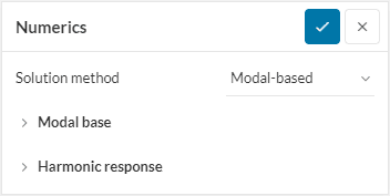
- Running modal-based harmonic? Use modal damping. Assigning ζ per mode is the most controllable option available, and it decouples damping from any assumption about how energy distributes spatially. If you have test data per mode, this is where it goes.
- Running harmonic on a material with real internal friction? Structural (hysteretic) damping models frequency-independent energy loss per cycle, which viscous models don’t. Restricted to the frequency domain, because the complex-modulus formulation presupposes harmonic motion.
- Screening or comparing variants? Global damping as a percentage of critical. Keep it below 15%, since harmonic analysis assumes the system oscillates. Fine for ranking designs, not defensible in a qualification package.
Get the Rayleigh coefficients right
Rayleigh damping builds C as a weighted sum of M and K, which keeps the equations decoupled in modal coordinates and makes them cheap to solve. That’s the whole reason it dominates. The cost is that ζ varies with frequency, and you only get to pin it at two points.
$$ \mathbf{C} = \alpha\mathbf{K} + \beta\mathbf{M} $$
$$ \zeta(\omega) = \frac{1}{2}\left(\alpha\omega + \frac{\beta}{\omega}\right) $$
Check the convention before you copy a coefficient
SimScale attaches α to the stiffness matrix. Abaqus and Ansys attach α to the mass matrix. Copying a coefficient across without swapping will be wrong by orders of magnitude at every frequency but one.
This is the single most common way a Rayleigh setup goes wrong, and it produces a model that runs cleanly and reports garbage.
| Tool | Damping matrix | α is | β is |
|---|---|---|---|
| SimScale | C = αK + βM | Stiffness-proportional [s] | Mass-proportional [1/s] |
Abaqus (*DAMPING) | C = αM + βK | Mass-proportional [1/s] | Stiffness-proportional [s] |
Ansys (ALPHAD / BETAD) | C = αM + βK | Mass-proportional [1/s] | Stiffness-proportional [s] |
| Clough and Penzien, Chopra | C = a₀M + a₁K | Mass-proportional | Stiffness-proportional |
One caveat worth knowing before you go looking: SimScale’s damping documentation and its Rayleigh coefficients guide both put α on the stiffness matrix in seconds, but at least one validation case lists the units the other way around. Trust the documentation page, and verify your coefficients reproduce a known ζ at a known frequency before you commit a long run to them.
Anchor at two frequencies, then check the dip
For a target ζ applied at two frequencies ω₁ and ω₂, in SimScale’s convention:
$$ \alpha = \frac{2\zeta}{\omega_1 + \omega_2}, \qquad \beta = \frac{2\zeta\,\omega_1\omega_2}{\omega_1 + \omega_2} $$
SimScale’s guide to computing Rayleigh coefficients derives these in full. Three behaviors fall out:
- β only (mass-proportional). ζ falls as frequency rises. Low modes get heavily damped, high modes ring.
- α only (stiffness-proportional). ζ rises with frequency. High-frequency content gets crushed, low modes ring. In an explicit transient run, heavy stiffness-proportional damping also shrinks the stable time step.
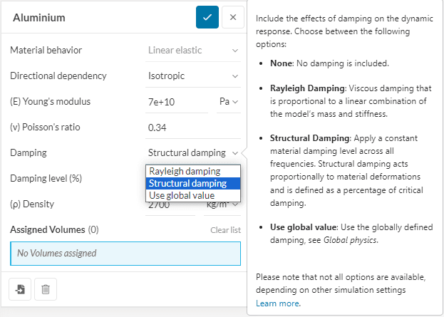
- Both. ζ is convex in frequency, with its minimum at the geometric mean of your two anchors, ω = √(β/α) = √(ω₁ω₂).
That minimum is the trap, and it’s worth working a number. Anchor at 10 Hz and 200 Hz targeting ζ = 2% and you get α = 3.03 × 10⁻⁵ s and β = 2.39 s⁻¹. Both anchors return exactly 2%. But the minimum sits at √(10 × 200) = 44.7 Hz, where ζ drops to 0.85%, well under half the target. Every mode between your anchors is under-damped, and the wider you space them the worse it gets: the ratio of achieved to target damping at the dip is just the geometric mean over the arithmetic mean of the anchor pair.
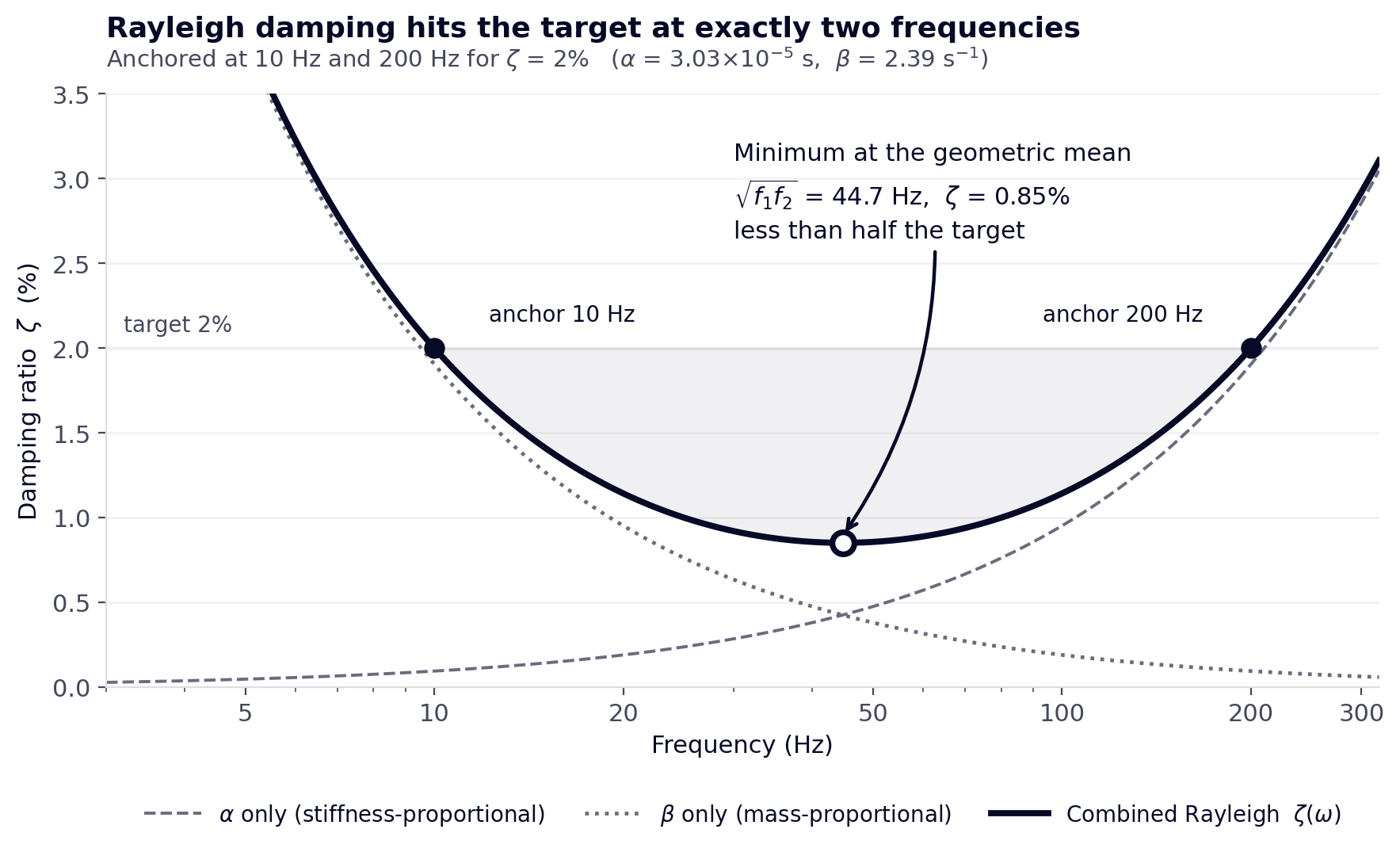
So if the mode carrying your response sits mid-band, spanning the full extraction range under-damps the one mode that matters, and your peak stresses come back high. Anchor tight around the modes actually carrying response instead.
No choice of α and β holds ζ constant across a band. For genuinely broadband excitation, either accept the error and document it, or move to modal damping.
Starting values, and what they’re worth
Use these as a first pass, not as a justification. Every row is amplitude- and construction-dependent, and the spread within a row is often larger than the difference between rows.
| Structure | Typical ζ | Notes |
|---|---|---|
| Bare aluminum, material only | 0.001% to 0.01% | Loss factor 1e-5 to 1e-4 |
| Bare steel, material only | 0.01% to 0.05% | |
| Welded steel structure | 0.1% to 0.5% | Welds add little |
| Fiber-reinforced composite | 0.2% to 2% | Depends on layup and matrix |
| Bolted steel structure, low amplitude | 0.5% to 2% | Rises sharply with amplitude |
| Prestressed concrete | 1% to 3% | Lower if uncracked |
| Reinforced concrete | 2% to 5% | |
| Assembly with many bolted joints | 2% to 7% | Requires joints free to micro-slip |
| Elastomeric mounts, rubber isolators | 5% to 20% |
Two structural facts drive everything in that table. Bulk metal barely damps: the material rows are two to three orders of magnitude below the assembly rows, so damping in a metal structure comes almost entirely from joints, welds, coatings, and boundary conditions. And joint damping depends on micro-slip, which means closely spaced, heavily torqued bolts contribute far less than the row suggests, while the same joint at seismic amplitude can double or triple its contribution once macro-slip sets in.
Two conventions are worth memorizing. Seismic response spectrum analysis assumes 5% of critical, and ASCE 7’s design spectra are defined at that value. Electronics vibration qualification generally runs 2% to 5% for housings and brackets.

Where the number is uncertain and the result matters, sweep it. A parametric study across the plausible range costs a handful of solves and tells you whether the design decision is even sensitive to ζ. Often it isn’t, which ends the argument.
Measure it instead
Two methods cover most cases, and both work off data you can get from a single accelerometer.
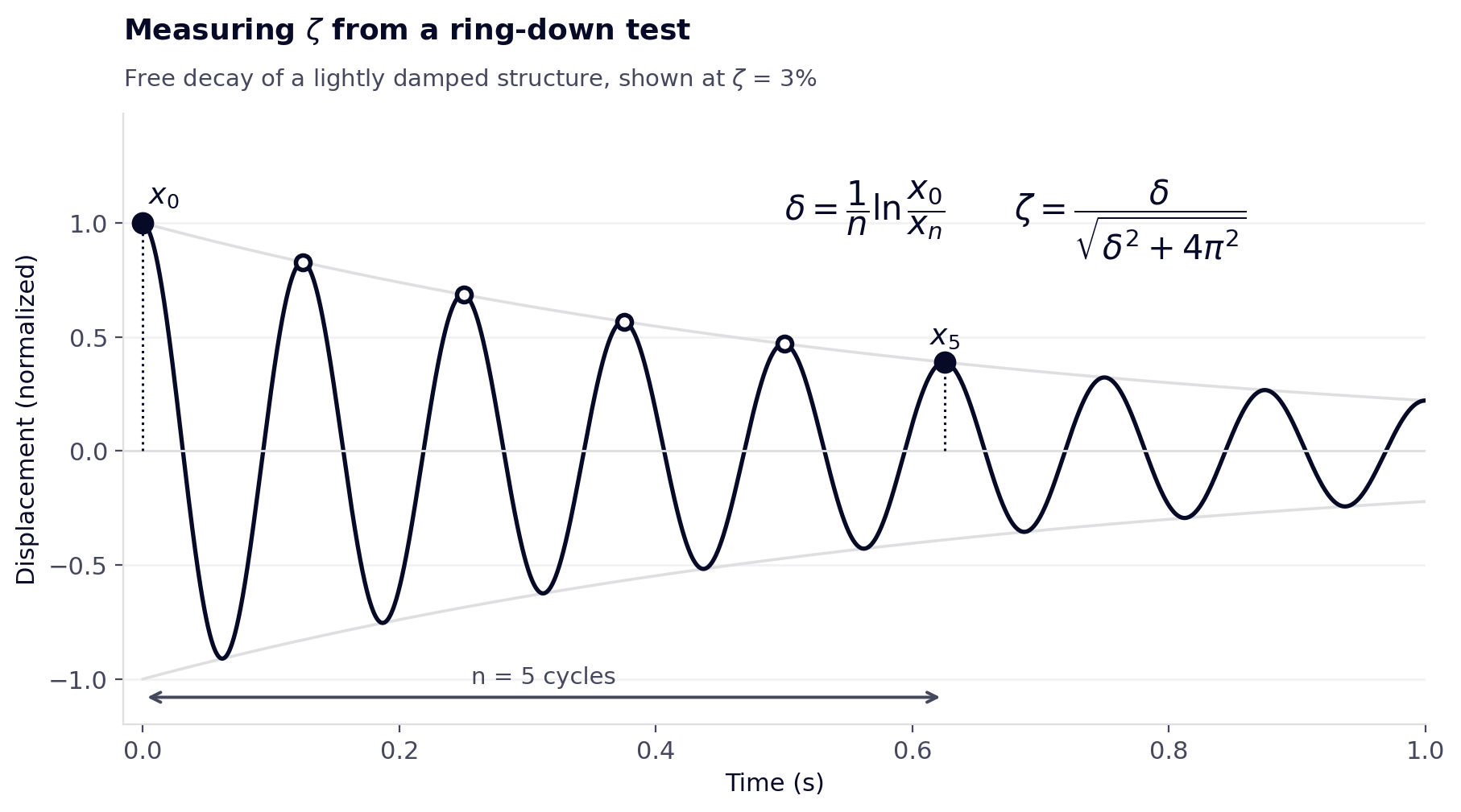
Logarithmic decrement, from a ring-down. Displace, release, measure successive peaks:
$$ \delta = \frac{1}{n}\ln\frac{x_0}{x_n}, \qquad \zeta = \frac{\delta}{\sqrt{\delta^2 + 4\pi^2}} $$
Use peaks n cycles apart rather than adjacent ones. On a lightly damped structure adjacent peaks differ by less than the noise floor, and the n-cycle form is the difference between a usable number and a meaningless one. For light damping this collapses to ζ ≈ δ/(2π).
Half-power bandwidth, from a sweep. Take the two frequencies either side of the peak where response falls to 1/√2 of maximum:
$$ \zeta = \frac{f_2 – f_1}{2 f_n} $$
Two failure modes. This is a light-damping approximation, not an identity, and it carries real error above ζ ≈ 0.1. More often, it breaks on closely spaced modes, where neighboring peaks contaminate the bandwidth and inflate the apparent damping. If your modes are within a few percent of each other, use curve fitting over the FRF instead of reading half-power points off it.
If you’re working from a published loss factor rather than a test, ζ = η/2, but only at resonance. Applying that conversion across a band introduces error that grows with distance from the anchor frequency.
Correlate the model before you trust the harmonic results
Run modal first, correlate against measurement, then run harmonic. Adjusting damping to match a measured FRF is the only way to arrive at a value you can defend, and it usually takes one instrumented unit.
Crestline Coach carries the auxiliary HVAC condenser above the cab on its ambulances, so a heavier condenser on a new build left the mounting bracket less stiff and more exposed to road input. Conlan Kirk on the New Product Development team ran modal analysis on the original sheet metal bracket and found natural modes below 100 Hz, inside the high-power vibration range.
He then cross-referenced against accelerometer data from a vehicle in the field. Two adjustments closed the gap: 2% global damping, and representing the condenser as a point mass rather than meshed geometry. That combination correlated the model to the measured behavior. Only then did the harmonic run mean anything, and it exposed a stress concentration at a weld joint caused by a sweep geometry amplifying stress under lateral sway. Adding a flange and swapping an L-channel for a stiffer profile moved the lowest vertical mode from 18 Hz to 147 Hz.
Note the order and the mass modeling. The damping ratio wasn’t the only correction; a point-mass idealization of the condenser mattered as much. Correlation failures often get blamed on damping when the real error is in mass distribution or boundary stiffness. Check those before you tune ζ to force a match, or you’ll bury a modeling error inside a damping value.
Don’t mistake numerical damping for physical damping
Dissipative time integration schemes remove energy from a transient solve independently of anything you set as material damping. That’s useful for suppressing spurious high-frequency oscillation and getting a nonlinear run to converge, and it’s a problem if you read the resulting amplitudes as physical.
The tell is a solution that changes when you refine the time step while everything else stays fixed. Energy conservation isn’t guaranteed under a dissipative scheme, so the amount removed depends on step size and on the frequency content the mesh resolves. Before trusting transient amplitudes, run the same case with a non-dissipative scheme, or halve the time step and confirm the peak response is stable. If it moves, the number you’re reading is partly an artifact of the integrator, not the structure.
Damping values from published qualification work
Three SimScale cases show what engineers actually specify: 5% for aerospace electronics qualification, 2% for a road-vehicle bracket correlated to field data, and modal response signatures for validating a damper design.
TechSAT qualifies airborne electrical equipment to RTCA DO-160G, which demands survival across 10 to 2000 Hz. Rather than replicate the full test in hardware, the team ran worst cases first: a modal analysis of an electronics housing returned 46 eigenfrequencies inside the band, then harmonic excitation at 10g at the fixing points with a 5% global damping ratio gave about 0.2 mm total displacement. Comparing two fixing strategies, the full rack support cut PCB deflection 18%, and the deflection map told them which regions of the board couldn’t carry high-inertia components.
Pektron checks every custom test jig for natural resonances before it goes on a shaker, since a jig resonating at the test frequency amplifies the input and destroys the unit under test. UKAS accreditation requires it. Modal analysis on STEP imports let them consolidate two jigs into one: “We’ve only had to build one jig to cover two jobs with the use of SimScale,” notes Andrew, “significantly reducing custom machining costs and physical laboratory setup time.”

Optimized Solutions designs the damper rather than working around one, developing an elastomer-based low-stiffness torsional vibration damper. Rubber torsional dampers handle high-frequency attenuation well but tend to be structurally unstable or ineffective at low frequency, so the design had to satisfy both. The model was heavily nonlinear: 10 degrees of angular deflection, hyperelastic material, 3D contact. The modal response signature is what proved low-frequency attenuation, and the frequency analyses ran in under 10 minutes on 4 cores.
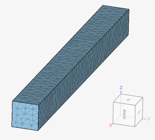
For solver verification, the straight beam with Rayleigh damping validation case checks displacement, velocity, and acceleration at the beam midpoint against Code_Aster and Europlexus reference results. Three public projects are open to copy: harmonic analysis of bearing tolerances in an impeller, a jet engine mount harmonic response study, and an EV battery modal and harmonic shaker-table model.
Run harmonic and nonlinear dynamic analyses in the browser
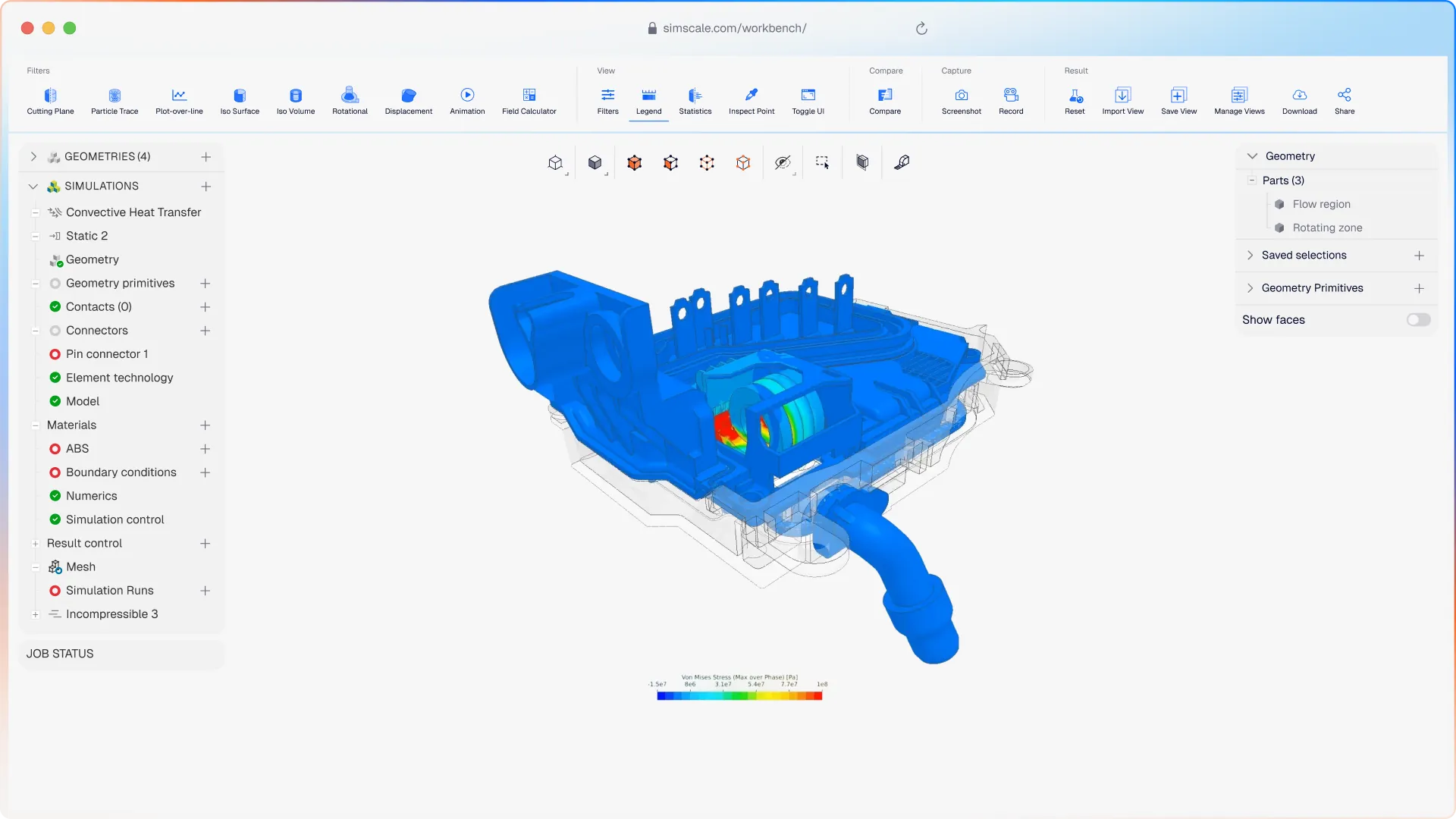
No HPC to provision, no install. Elastic compute and all physics in one platform.
Frequently asked questions
Rayleigh, because it’s the only one available. Modal and structural damping both presuppose a fixed modal basis or harmonic motion, neither of which survives a changing tangent stiffness. Some codes let you back Rayleigh coefficients out of a target modal damping ratio for direct integration, which is a convenience, not equivalent to modal damping. Watch the stable time step if you’re using stiffness-proportional damping in an explicit solve.
Swap them. SimScale uses C = αK + βM with α stiffness-proportional in seconds; Abaqus and Ansys use C = αM + βK with α mass-proportional in 1/seconds. SimScale’s α is the other tool’s β and vice versa. Rather than relying on the swap alone, recompute from the underlying physical target: take your two anchor frequencies and target ζ, and solve for the coefficients in whichever convention the destination solver uses.
The viscous damping coefficient c is N·s/m, dimensionally kg/s, or N·m·s/rad for rotational systems. The damping ratio ζ is dimensionless. For Rayleigh coefficients, the stiffness-proportional coefficient has units of seconds and the mass-proportional coefficient units of 1/seconds, regardless of which one your solver calls α.
Because ζ(ω) is convex when both coefficients are active, with a minimum at ω = √(β/α) in SimScale’s convention. Anchoring at two frequencies with equal target damping guarantees every mode between them is damped below target. Move the anchors in tight around the modes actually carrying response, or switch to modal damping if the band is genuinely wide.
Refine the time step and see whether the peak amplitude moves. Physical damping is step-size independent; numerical dissipation isn’t. Re-running with a non-dissipative integration scheme isolates it directly. Any amplitude that shifts under time-step refinement is partly an integrator artifact.
0.1% to 0.5% for welded steel, 2% to 5% for a bolted electronics housing, 5% for seismic response spectrum work. Then sweep it across the plausible range instead of defending a single value. If the design decision flips inside that range, you need a measurement; if it doesn’t, document the sweep and move on.
Not meaningfully at structural damping levels. ω_d = ω_n√(1 − ζ²), so at ζ = 0.05 the damped frequency is 99.87% of the undamped value. That’s why eigenfrequency extraction ignores damping. Response amplitudes are a different matter entirely, and that’s where the value earns its attention.