
Undersize a pump and the top floor runs dry. Oversize it and you pay for that mistake on every electricity bill for the next 20 years. Both come down to one number most engineers estimate too late: major head loss, the pressure a fluid burns off to friction as it travels a straight run of pipe or duct.
You calculate it with the Darcy-Weisbach equation, \(h_f = f \times \frac{L}{D} \times \frac{v^2}{2g}\), where the friction factor \(f\) comes from the flow regime and the pipe’s roughness. The math is quick. Getting the inputs right, the friction factor, the real roughness of an aged pipe, the velocity at peak demand, is where designs go wrong.
Head loss comes in two parts:
- Major head loss: friction along straight runs. Usually the larger share in long pipe and duct systems.
- Minor head loss: local losses at valves, fittings, and bends.
This article covers the major component in depth and shows where the minor losses fit, so you can size the full system. We’ll work through the hand calculation, then show what CFD in SimScale adds once the geometry gets real: branching networks, fouling, temperature-driven viscosity changes.
What Is Head Loss?
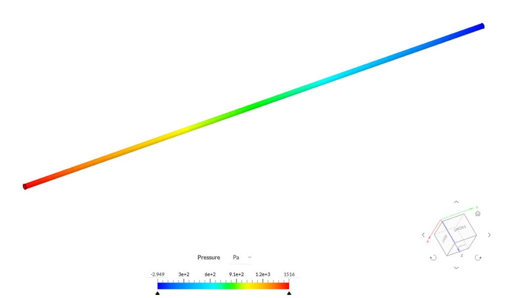
Head loss is the irreversible loss of fluid energy to friction and turbulence, expressed as an equivalent height of fluid column. The units are length: meters in SI, feet in imperial. A head loss of 5 m means the friction over that run costs the same energy as lifting the fluid 5 m against gravity.
Major head loss (\(h_f\)) is the share caused by friction along straight pipe walls. It grows with pipe length, fluid velocity, and surface roughness, and it shrinks as pipe diameter grows. Minor head loss covers the rest, the local disruptions at fittings and components.
Units of Head Loss
Head loss is always a length, because it represents energy per unit weight of fluid. In SI units that’s meters of fluid column (m); in imperial units it’s feet (ft). To convert head loss to a pressure drop, multiply by fluid density and gravity (covered below). Don’t confuse head loss (m or ft) with pressure drop (Pa, bar, or psi). They describe the same energy loss in different terms.
Calculating with the Darcy-Weisbach head loss formula
The Darcy-Weisbach equation is the standard way to calculate major head loss, valid for any fluid in any flow regime. Named after hydraulic engineers Henry Darcy and Julius Weisbach, it relates head loss to fluid properties, pipe dimensions, and flow characteristics, so you can size systems for the efficiency you need. It’s written as:
$$ h_f = f \times \frac{L}{D} \times \frac{v^2}{2g} $$
Where:
- \(h_f\) = head loss due to friction (m or ft)
- \(f\) = Darcy friction factor (dimensionless)
- \(L\) = length of the pipe (m or ft)
- \(D\) = diameter of the pipe (m or ft)
- \(v\) = fluid velocity (m/s or ft/s)
- \(g\) = gravitational acceleration, 9.81 m/s²
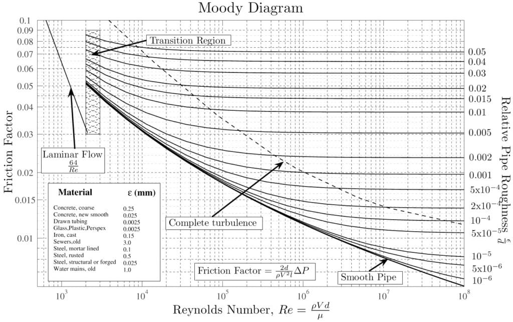
The friction factor depends on the flow regime, which the Reynolds number sets. For laminar flow, \(f\) follows directly from the Reynolds number. For turbulent flow, it depends on both the Reynolds number and the pipe’s relative roughness, and engineers reach for the Moody chart, a graphical plot of friction factor against Reynolds number and relative roughness. Read off the friction factor at your point on the chart and the rest of the calculation is arithmetic.
Apply Darcy-Weisbach correctly and you can predict frictional losses and design systems that run reliably with minimal wasted energy. Simulation tools like SimScale take it further by modeling the fluid behavior directly and validating the head loss across the real geometry, which sharpens both the speed and the precision of the design.
Step-by-Step guide to Calculating Major Head Loss
Calculating major head loss takes a few ordered steps: identify the flow regime, find the friction factor, then apply the Darcy-Weisbach equation. Here’s each one.
1. Determine the Flow Regime
Start by calculating the Reynolds number \(Re\), the dimensionless ratio that tells you whether the flow is laminar or turbulent. That classification decides how you find the friction factor. Use:
$$ Re = \frac{v \times D}{\nu} $$
Where \(\nu\) is the kinematic viscosity of the fluid.
- If \(Re < 2000\), the flow is laminar.
- If \(Re > 4000\), the flow is turbulent.
- Between 2000 and 4000, the flow is transitional and needs care.
Transitional flow can shift between laminar and turbulent behavior, so small changes in conditions move the answer. For these cases:
- Run stability checks. Test whether small changes in conditions push the flow one way or the other, with extra testing or simulation if the design is sensitive.
- Use conservative estimates. A friction factor closer to the turbulent value adds a safety margin where pressure control matters.
- Use CFD. SimScale CFD models transitional flow more accurately than a single chart value, which helps when the standard equations sit at their limits.
- Iterate. Try both laminar and turbulent friction factors, see which gives the more realistic estimate, and adjust the design around it.
2. Calculate the Friction Factor \(f\)
The method depends entirely on the regime you found in step 1.
For laminar flow, the friction factor comes straight from the Reynolds number, no chart needed:
$$ f = \frac{64}{Re} $$
For turbulent flow, the friction factor depends on both the Reynolds number and the pipe’s relative roughness. The Colebrook-White equation is the standard, though it has to be solved iteratively:
$$ \frac{1}{\sqrt{f}} = -2 \log \left( \frac{\epsilon}{3.7D} + \frac{2.51}{Re \sqrt{f}} \right) $$
Here \(\epsilon\) is the absolute roughness of the pipe material. To skip the iteration, read \(f\) off a Moody chart using \(Re\) and the relative roughness \(\epsilon/D\).
Typical Absolute Roughness Values
The roughness \(\epsilon\) you plug into Colebrook-White or the Moody chart depends on the pipe material:
| Material | Absolute roughness ε (mm) |
|---|---|
| Drawn tubing (copper, brass, glass) | 0.0015 |
| Commercial steel / welded steel | 0.045 |
| Galvanized iron | 0.15 |
| Cast iron (new) | 0.26 |
| Concrete | 0.3 to 3.0 |
| Riveted steel | 0.9 to 9.0 |
Roughness grows over a system’s life as scale, corrosion, and fouling build up, so design with a margin rather than the new-pipe value alone.
3. Substitute Values into the Darcy-Weisbach Equation
With the friction factor \(f\), pipe length \(L\), diameter \(D\), and velocity \(v\) in hand, drop them into the equation:
$$ h_f = f \times \frac{L}{D} \times \frac{v^2}{2g} $$
The result is the major head loss in meters or feet, depending on your unit system, a direct measure of the energy lost to friction over that run.
4. Adjust for Unit Consistency
Keep every unit in the same system before you calculate. If velocity is in meters per second and diameter is in meters, then \(g\) has to be 9.81 m/s². Mixing SI and imperial midway through is the most common source of a wrong answer.
Major vs minor losses in pipe flow
The Darcy-Weisbach calculation above gives you major head loss, the friction along straight pipe. But a real system also loses energy at every valve, elbow, tee, expansion, and contraction. Those are the minor losses, and in a system with many fittings they add up to anything but minor.
The difference is where the loss happens:
- Major losses occur along straight runs, driven by wall friction. They scale with length, so they dominate in long pipelines and duct runs.
- Minor losses occur at local components, driven by flow separation and turbulence as the fluid changes direction or speed. They dominate in short, fitting-heavy systems like pump skids and manifolds.
Minor losses use the loss-coefficient (K-factor) method:
$$ h_m = K \times \frac{v^2}{2g} $$
Each component has a characteristic K value: roughly 0.9 for a standard 90° elbow, 0.2 for a gate valve fully open, up to 10 for a globe valve fully open. The pressure drop across components like a globe valve or any fitting with a flow coefficient is a minor loss in this sense.
Total Head Loss
Total head loss in a system is simply the sum of both parts:
$$ h_{total} = h_{major} + h_{minor} = \left( f \frac{L}{D} + \sum K \right) \frac{v^2}{2g} $$
You need the total, not just the major component, to size a pump correctly. Calculate the major loss along each straight run, add the K-factor losses for every fitting, and sum them across the flow path.
Example: Major Head Loss Calculation
An engineering team is designing a water distribution system for a small residential area. The system has to deliver consistent pressure to every home, so the head loss in the main supply pipe decides whether the far houses get enough pressure. The team has these parameters:
- Pipe length \(L = 100 \, m\)
- Pipe diameter \(D = 0.3 \, m\)
- Water velocity \(v = 1.5 \, m/s\)
- Pipe roughness \(\epsilon = 0.00015 \, m\) (commercial steel)
- Water kinematic viscosity \(\nu = 1 \times 10^{-6} \, m^2/s\)
The goal is the major head loss in this pipe section, so they can confirm the spec.
Solution
1. Calculate the Reynolds number.
$$ Re = \frac{v \times D}{\nu} = \frac{1.5 \times 0.3}{1 \times 10^{-6}} = 450{,}000 $$
Since \(Re > 4000\), the flow is turbulent.
2. Determine the friction factor \(f\).
For turbulent flow, the friction factor depends on the Reynolds number and the relative roughness. Using the Colebrook-White equation or a Moody chart gives \(f \approx 0.02\).
3. Calculate the major head loss.
$$ h_f = f \times \frac{L}{D} \times \frac{v^2}{2g} = 0.02 \times \frac{100}{0.3} \times \frac{1.5^2}{2 \times 9.81} = 0.76 \, m $$
The major head loss in this pipe section is \(h_f \approx 0.76 \, m\).
This is the friction loss over the 100 m run. It tells the team whether they need a larger diameter, a shorter route, or more pumping power to hold pressure across the network. In a full system study they’d add the minor losses from every valve and bend to get the total head the pump has to overcome.
Head Loss vs Pressure Drop: How to Convert
Head loss and pressure drop describe the same energy loss in different units. Head loss is a length (m or ft); pressure drop is a force per area (Pa, bar, or psi). Convert between them with:
$$ \Delta P = \rho \times g \times h_f $$
Where \(\rho\) is fluid density (kg/m³), \(g\) is 9.81 m/s², and \(h_f\) is head loss in meters. The result is in pascals.
Take the example above. With water at \(\rho = 1000 \, kg/m^3\) and \(h_f = 0.76 \, m\):
$$ \Delta P = 1000 \times 9.81 \times 0.76 \approx 7{,}460 \, Pa \approx 0.075 \, bar $$
Pump curves are usually quoted in head, while instrumentation and spec sheets often read in pressure, so engineers convert between the two constantly. For the simulation side of this, see SimScale’s guidance on pressure drop best practice for internal flows.
Alternative Head Loss Formulas: When to Use Each
Darcy-Weisbach is the universal method, valid for any fluid across laminar and turbulent flow. But two empirical formulas show up often enough in practice that it’s worth knowing when each fits.
| Method | Best for | Trade-off |
|---|---|---|
| Darcy-Weisbach | Any fluid, any regime, any pipe | Most accurate, but needs the friction factor (iterative or Moody chart) |
| Hazen-Williams | Water in pressurized pipes, ~4 to 25 °C | Simple, non-iterative, but water-only and temperature-limited |
| Manning / Chezy | Open-channel and gravity flow | Built for free-surface flow, not full pressurized pipe |
The Hazen-Williams equation skips the friction factor entirely and uses a roughness coefficient \(C\) instead (around 150 for new PVC, 130 for new steel, 100 for older cast iron). It’s the standard in water utility and fire-protection design because the math is quick and the fluid is always water near ambient temperature. Outside those conditions, Darcy-Weisbach is the safer choice because it accounts for viscosity and the full range of flow regimes.
Factors Affecting Major Head Loss
The Darcy-Weisbach equation shows that major head loss depends on pipe diameter, length, fluid velocity, pipe roughness, and fluid viscosity. Each one shapes the friction-driven pressure drop and, through it, the system’s efficiency, energy use, and maintenance cost.
Pipe Diameter
Smaller diameters raise head loss sharply, because friction matters more relative to the flow area. At high flow rates a narrow pipe causes large pressure drops, cutting efficiency and forcing larger pumps. Engineers balance diameter against material cost and available space; for critical systems, a larger diameter lowers head loss and pump load and pays back in energy over the system’s life.
Pipe Length
Longer pipes accumulate more friction, so head loss rises with length. In systems spanning long distances, like municipal water networks, length drives a large share of the energy requirement. Trimming unnecessary runs or adding intermediate pump stations keeps the flow efficient and the energy cost down.
Fluid Velocity
Head loss grows with the square of velocity, so doubling speed roughly quadruples the friction loss. Higher velocities move more fluid but demand more energy and accelerate wear on pipes and fittings. Engineers set velocity limits that balance throughput against cost and erosion.
Pipe Roughness
Surface roughness sets the friction factor in turbulent flow. Rough materials like cast iron create more friction and higher head loss; smoother materials like PVC or stainless steel cut it. For systems where head loss is critical, such as high-precision HVAC or water distribution, smoother pipe keeps energy use low. Roughness also climbs as surfaces degrade, so maintenance matters over time.
Fluid Viscosity
Viscosity changes little in water systems but dominates with oils, chemicals, and other viscous fluids, where higher viscosity raises resistance and head loss. For viscous service, engineers often choose larger diameters or lower flow rates to compensate. Because temperature shifts viscosity strongly, the operating temperature has to feed into the calculation.
Together these factors drive both system design and running cost. Reading how diameter, length, velocity, roughness, and viscosity interact lets engineers cut energy use and keep systems reliable for their full life. SimScale models all of them at once, so you can test design scenarios and find the lowest-head-loss configuration before anything is built.
Optimizing Major Head Loss Calculations with SimScale
Simulation predicts head loss across the real geometry, where a single formula can’t: branching networks, fouling, weld roughness, temperature swings. SimScale lets engineers visualize, refine, and optimize the whole system before anything is built. Six ways it goes beyond the hand calculation:
1. Visualize Flow and Pressure Distribution
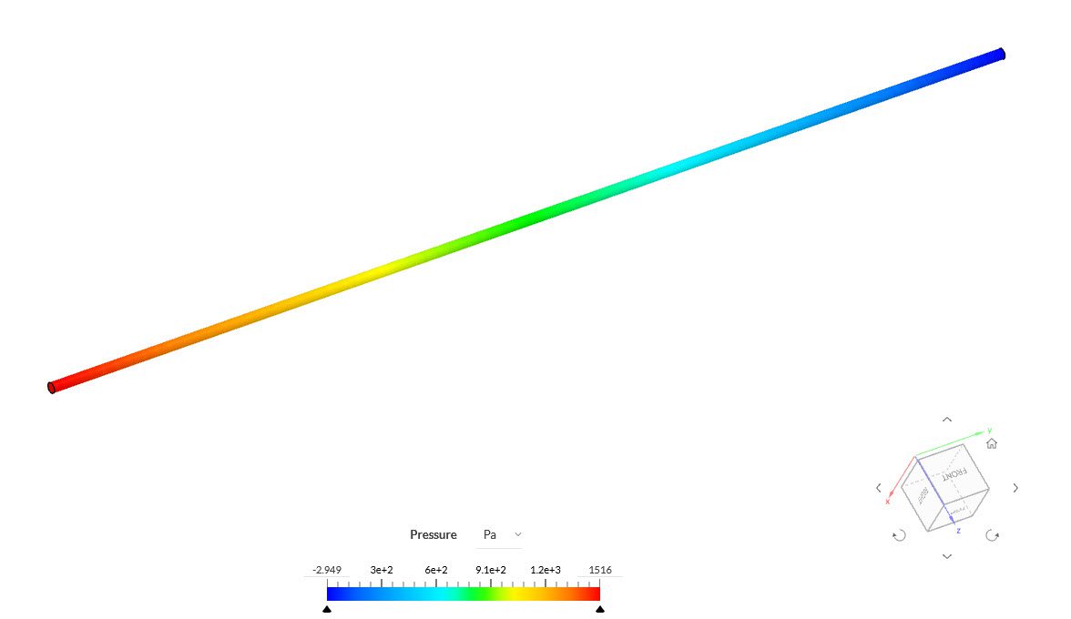
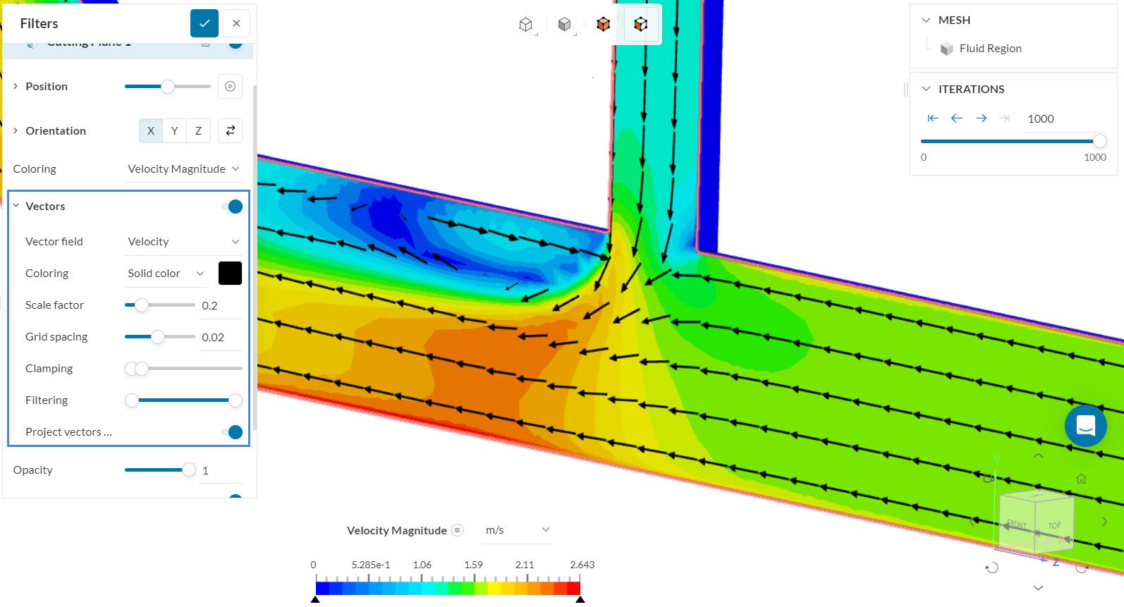
SimScale simulates flow across a full piping network and provides the full pressure and velocity fields directly. The high-loss regions are easy to see in 1D or 2D scalar plots, which points you straight at the design changes that help: resize a run, swap a material, modify a bend.
2. Refine Friction Factor Calculations
Pinning down the friction factor by hand is awkward for turbulent and transitional flow. Feed SimScale the pipe roughness, Reynolds number, and flow conditions and it resolves the friction behavior inside the solve, so you get head loss across varied conditions without separate manual friction-factor work.
3. Test Multiple Scenarios at Once
On SimScale’s cloud-native platform you run many simulations in parallel and compare designs side by side. Sweep pipe diameters, lengths, or materials in one study and find the configuration that minimizes head loss while still meeting performance and cost targets.
4. Account for Temperature-Dependent Fluid Properties
SimScale handles temperature variation and its effect on properties like viscosity. That matters wherever temperature influences fluid behavior, from HVAC systems to industrial lines carrying oils or chemicals, and it keeps the predicted performance honest across operating conditions.
5. Catch Design Errors Before Rework
Modeling head loss early surfaces inefficiencies before anything is built. That helps to avoid underperforming systems, excess energy use, and expensive late changes, because the design decisions rest on accurate simulation rather than rough estimates.
6. Scale to Complex Systems with Confidence
For large systems, like municipal water networks or extensive industrial pipelines, head loss across many segments is hard to track by hand. SimScale simulates the whole network and shows the head-loss distribution across it, so critical components get sized right and pump strain stays in check.
What Engineers Have Achieved with SimScale
The payoff shows up as real pressure-drop reductions:
- Diinef cut the pressure drop across a hydraulic motor valve by 80% with CFD, bringing it into the target operating range and steering the cavitation zone away from the wall. See the Diinef case study.
- ATAG reduced the pressure drop through their exhaust piping by 70% after CFD studies showed where flow reinforcements were creating eddies. See the ATAG case study.
To see the major-loss calculation run as a simulation, the public project Pressure Drop in Turbulent Flow through a Pipe models airflow through a straight smooth pipe at five velocities and checks the CFD result against the analytical value.
Frequently Asked Questions
The major head loss formula is the Darcy-Weisbach equation: \(h_f = f \times \frac{L}{D} \times \frac{v^2}{2g}\), where \(f\) is the friction factor, \(L\) the pipe length, \(D\) the diameter, \(v\) the fluid velocity, and \(g\) gravitational acceleration. It gives head loss as a length of fluid column.
Major head loss is friction along straight pipe and scales with length. Minor head loss is the local loss at valves, fittings, and bends, calculated with the K-factor method \(h_m = K \frac{v^2}{2g}\). Total head loss is the sum of both.
Head loss is a length: meters of fluid column in SI, feet in imperial. It represents energy lost per unit weight of fluid. Multiply by \(\rho g\) to convert it to a pressure drop in pascals.
Find the Reynolds number to set the flow regime, get the friction factor (\(f = 64/Re\) for laminar, Colebrook-White or the Moody chart for turbulent), then substitute the friction factor, length, diameter, and velocity into the Darcy-Weisbach equation.
Use Darcy-Weisbach for any fluid and any flow regime; it’s the universal, most accurate method. Use Hazen-Williams as a quick shortcut for water in pressurized pipes near ambient temperature, common in water-utility and fire-protection design.
Conclusion
Managing major head loss well is what keeps a fluid system efficient and reliable over its life. The Darcy-Weisbach equation gets you a sound theoretical number, and adding the minor losses gives you the total head a pump has to overcome. For real networks with branching, fouling, and temperature effects, SimScale takes you past hand calculation: model the actual flow, find the high-loss regions, and tune the design against real conditions. With cloud-native compute and parallel runs, you can explore many configurations at once and size the system right before it’s built.