Fill out the form to download

Required field
Required field
Not a valid email address
Required field
Required field

Fill out the form to download

Required field
Required field
Required field
Required field
Required field
Required field
Required field
Required field

Thank you. We will contact you shortly.

  • Set up your own cloud-native simulation in minutes.

  • When Is It Just a Pretty Picture? Tips For a Better Structural Analysis

    Christopher Quijano
    BlogFEAWhen Is It Just a Pretty Picture? Tips For a Better Structural Analysis

    Structural analysis has come a long way since the days of punch cards and line printers. The easy access to CAD data, increased capabilities of the tools, and “wizards” that walk users through the process have all contributed to the increased growth of the simulation industry.

    In the early days of finite elements, analysts would review pages and pages of printed tabular results. Now, with a mere click of a button, we can produce a beautifully contoured color plot. We can visualize the finite element results in the larger assembly, and we are approaching the point with the advent of virtual reality, that we can walk through our results and interact with the assembly virtually. These capabilities make it easy to create stunning and very convincing pictures, but also make it very easy to believe inaccurate results.

    Anyone with experience with simulation has had that “oops” moment. Particularly when results have been presented, the product has been manufactured, and a part fails in service. Reverting to the structural analysis, you realize that a mistake has been made. If you are lucky no one gets injured or dies, and if you are really lucky the product has margin and no changes need to be made.

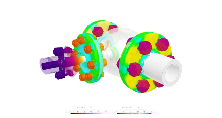
    structural analysis bolted connection von mises stress analysis and fea simulation
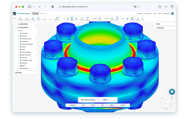
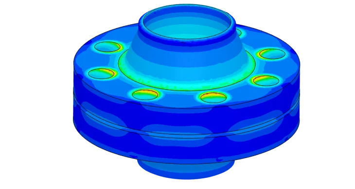
    FEA of bolted connection carried out with SimScale

    If you are not so lucky, the consequences can be dire. One such example is the Sleipner A offshore oil platform. In 1991, this platform underwent a controlled ballasting test when a failure occurred and it sank to the ocean floor. The Sleipner A was designed using extensive finite element analysis and this was performed using a reputable commercial code (Nastran). The failure investigation determined that the stresses in the ballast chamber were underestimated by 47%, causing an under-design of the ballast walls which subsequently weren’t thick enough to support the pressures.

    To minimize the errors in a simulation, the analyst needs to have a very good understanding of the loads and how they affect the model, and also be aware of the assumptions made in CAD and the structural analysis tools. Finally, the analyst needs to understand the limitations of the technology used.

    Sources of Errors in Structural Analysis

    The main sources of error in simulation typically fall into one of the following categories:

    • CAD geometry/simplifications
    • Lack of understanding of the math/physics behind FEA
    • Lack of understanding of the real loads, materials, etc
    • Lack of understanding of the capabilities of the simulation tool

    Ben Lewis, the Managing Partner of Custom Machines, held a webinar covering the simplification of CAD for FEA purposes. Ben deals with large complex assemblies and this training is a good reference for how to properly prepare CAD data. Watch this webinar recording for free.

    In the SimScale forum, power user Jousef (@jousefm) has written several articles on the fundamentals of the math and physics behind the finite element method. Jousef’s articles are great if you are new to simulation or need a refresher on the math behind the magic.

    The rest of this article will focus on the SimScale tool, how it differs from other simulation tools and some tips on how to get more accurate structural analysis results. The topic will mainly be linear static, but the content applies to other types of structural analysis as well.

    Meshing

    meshing types of elements, line 1d elements spring damper beam truss, surface 2d elements shell plane2d, volume 3d elements hexahedral tetrahedral

    Once you have imported the geometry into SimScale, the next step is to apply a mesh to that geometry. Meshing the geometry refers to breaking down the parts or assembly into smaller pieces called elements.

    Let’s take a step back for a minute. In general, when creating a mesh, there is the option of choosing between 1D, 2D, or 3D elements. 1D is a line or a curve element, such as a spring or beam. 2D elements are used to mesh surfaces and the thickness needs to be specified. 3D elements are used to mesh solid volumes. The table on the right shows the various element types and the location of the nodes on each of them. The first order elements are linear. This refers to the linear interpolation used to calculate the values between the nodes. The second order elements use quadratic interpolation to calculate values between the nodes. In general, the latter delivers better results.

    Currently, for structural analysis, SimScale only supports the tetrahedral elements. While this does pose some limitations, which we will discuss later, a workaround using more elements at the cost of model size and solution time, can be found.

    Now that we understand what elements SimScale uses, we can look at the algorithms for actually meshing the model. SimScale provides four options for creating a structural mesh and you have to choose one before setting up the mesh parameters. The four options are outlined below:

    Tetrahedral Automatic is the most basic meshing algorithm. The user selects a first or second order mesh, and chooses between five options for the mesh size—from “Very Course” to “Very Fine”. This method is very good for the initial analysis to check the geometry, and gives the user a good idea of what areas need more refinement. Tetrahedral Automatic generally does a good job refining the mesh in areas of high curvature.

    Tetrahedral Parametric creates the same quality of mesh as Tetrahedral Automatic and has the same refinement in areas of high curvature. The main difference with Tetrahedral Parametric is that it allows the user to specify the global maximum and minimum element edge length. This allows more control of the overall element size. For example, if there is a thin part and multiple elements need to be forced through the thickness, this can be achieved by limiting the maximum element size to a fraction of the thickness. Or if a long part is needed where only the stresses at the end are of interest, the maximum element size can be increased.

    Tetrahedral with Local Refinements is the same as Tetrahedral Parametric but allows the selection of edges, surfaces, or volumes for localized refinement. With this method, the global minimum and maximum element size are specified and then a finer mesh is added to areas where more resolution is required.

    Tetrahedral with Layer Refinements resembles a tetrahedral CFD mesh. It begins with the Tetrahedral Automatic option but then allows automatic mesh refinement near the surfaces or faces of the mesh. The options include the total depth of the layers, the number of layers, and an expansion factor. While this does appear to produce good results, it’s not an option used often.

    SimScale Meshing Tips for Structural Analysis

    tet element

    Once meshing algorithms are understood, the meshing process is straightforward in SimScale. The main areas to watch are more specific to the tetrahedral element and not SimScale. Here are a few to consider:

    • One of the checks for the “goodness” of the tet element is called the “aspect ratio”. This is the ratio of the longest edge, over the shortest edge. In the areas where good results are required, the ration needs to be close to 1:1. In areas away from the areas of interest, the ratio can be 5:1 or slightly higher. The automatic mesher in SimScale works well and performs an internal test for the aspect ratio. If the aspect ratio required differs, the Tetrahedral with Local Refinements is a good way to change this around. In the post-processing, the element aspect ratios can be reviewed.
    • First order Tetrahedral elements tend to be overly stiff especially for bending problems. To account for this, a finer mesh or second order Tetrahedral elements is needed. first order mesh, second order mesh
    • In general, second-order Tet elements are recommended over first-order Tet elements for linear static analysis. First order Tet elements work well for thermal analysis. For contact analysis, second-order Tets can have difficulty converging.
    • Typically long thin sections such as sheet metal are better meshed with shell elements. Since SimScale only has Tetrahedral elements, the only option is to use solid elements. Thin sections under a bending load require approximately three to four linear elements through the thickness to resolve the stresses. Second order Tet elements can achieve this in one to two elements through the thickness.

    Solution Type and Solvers

    Once the mesh is created, the next step is to set up the structural analysis in the simulation designer. In the Solid Mechanics tab, there are two options: “physics perspective” and “solver perspective”.SimScale platform simulation analysis types

    This is because SimScale has integrated multiple solvers into the platform with potentially overlapping functionality. On the “physics perspective”, always choose the default solver for each analysis type. If a specific solver is required, a specific analysis type using the “solver perspective” can be chosen.

    For solid mechanics, there are currently two solvers integrated. One solver is Code_Aster, which is open source and developed by EDF. The other is CalculiX, which is also open source and developed by MTU Aero engines. The default type for all analysis types that are available for both solvers (Static, Dynamic, Heat transfer, and Thermomechanical) is Code_Aster.

    In the tables below are summaries of each solver’s advantages and disadvantages.

    Static Analysis

    Static

    (Using CalculiX via Solver Perspective)

    Static (default)

    Solver

    CalculiX

    Code_Aster

    Advantages

    • Faster solver
    • Can handle contact between a single body

    • Larger selection of boundary conditions
    • Larger selection of constraints
    • Loads and constraints based on tables or functions
    • Nonlinearity, geometric, material, time-dependent
    • Larger selection of results can be chosen
    • Results can be calculated based on points, edges, faces, or volumes

    Disadvantages

    • Limited to a fixed boundary condition
    • Loads are limited to nodal loads, pressure, torque
    • Results are only displacement, stress, strain
    • Linear only
    • Cannot handle contact between a single body (i.e. folded up sheet metal box)

    Dynamic Analysis

    Dynamic 

    (Using CalculiX via Solver Perspective)

    Dynamic

    Solver

    CalculiX

    Code_Aster

    Advantages

    • Faster solver
    • Can handle contact between a single body
    • Linear time-dependent solution

    • Larger selection of boundary conditions
    • Larger selection of constraints
    • Loads and constraints based on tables or functions
    • Nonlinearity, geometric, material, time-dependent, impact
    • Larger selection of results can be chosen
    • Results can be calculated based on points, edges, faces, or volumes

    Disadvantages

    • Limited to a fixed boundary condition
    • Loads are limited to nodal loads, pressure, torque
    • Results are only displacement, stress, strain
    • Linear only
    • Cannot handle contact between a single body (i.e. folded up sheet metal box)

    Vibration Analysis

    Frequency

    Modal

    Harmonic

    Solver

    CalculiX

    CalculiX

    Code_Aster

    Advantages

    Calculates:

     Eigenfrequencies

     Eigenmodes

     Effective Model Mass

    Calculates:

     Eigenfrequencies

     Eigenmodes

     Dynamic Response

    • Modal dynamics are based on the linearly superposed eigenmodes
    • Computationally less expensive

    Calculates:

     Structural response

      to periodic loads

    • Loading as a function of frequency
    • Includes damping
    • Results are a complex number

    Disadvantages

    • Does not perform any time-based calculations
    • Linear elastic only
    • Dependant on the number of modes requested
    • Linear elastic only
    • Computationally more expensive

    SimScale Structural Analysis Type Tip

    • The default Static and Dynamic analysis types do require slightly more input for setup, but they are the recommended solvers due to their more robust loading and boundary conditions.

    Loads and Boundary Conditions

    Loads and boundary conditions are the tools used to translate reality into a computer-solvable model. How they are defined, how well the results are understood, and the actual loads and boundary conditions will determine the accuracy of the model.

    For example, see the structure in Figure 1. If the maximum stress in the horizontal beam is of interest, the model in Figure 2 can be used and this will give good stress results. But if the maximum deflection is required, however, this model will be wrong. While the chosen boundary condition does allow for the correct stress, it is too rigid and causes errors in the displacement. This is a very simple example of how results can be correct and/or incorrect based on assumptions and boundary conditions.

    loaded beam, simplified beam

    Now that boundary conditions and how assumptions can affect the results is understood, a walk through the SimScale analysis is required.

    In the Domain section, there is an option for Contacts. In this area, Bonded contacts, Sliding contacts, or Cyclic Symmetry contacts can be defined. In many CAD-based simulation packages, a simple selection of the surfaces that require contact can be achieved. SimScale uses the more traditional terminology of Master and Slave surfaces. The master surfaces should be the larger, flatter, and stiffer surfaces and they should have the coarser mesh. The converse is true for Slave surfaces.

    Bonded contacts are just as the name implies, all of the Slave surfaces are fixed to the master surfaces as if it was a single part. The sliding contact constraints the Slave surfaces (nodes) to slide along the Master surfaces. The cyclic symmetry contact allows the modeling of a single segment of a fully-revolved part or assembly.

    SimScale Tip: For bonded contacts, the surfaces do not need to be touching. There is a tolerance option in the settings. Contacts follow the linear assumption for small displacements.

    If the Dynamic or Static analysis type is selected and set nonlinear to true, there will be an option for Physical Contacts. Physical contacts allow the modeling of the actual load path through joints, parts coming into contact, or penetration. Physical contacts need to be a separate topic.

    We will not discuss material properties, this area should be self-explanatory.

    In the Initial conditions section, SimScale allows the definition of an initial displacement or an initial stress. These options can be used to put in a pre-stress, for example.

    The loads and boundary condition areas are straightforward and comparable to other packages. Most loads can be entered as a value, table, or formula.

    While SimScale does not support Spring elements, it does have an Elastic Support boundary condition which can simulate one node spring to the ground element.

    Finally, SimScale offers a remote displacement and a remote force. These act as an RBE2 or RBE3 multipoint constraints. When they are set to undeformable, the remote point is rigidly attached to all nodes on the surfaces. When these are set to deformable, the transmitted displacement/load becomes a weighted average.

    SimScale Loads Boundary Conditions Tips

    • SimScale doesn’t attach loads and boundary conditions to the CAD geometry the way other simulation packages do. The loads and boundary conditions are applied to the mesh. So, when the model is re-meshed, the boundary conditions need to be attached again.
    • SimScale doesn’t support local coordinate systems for applying loads or boundary conditions. All loads and boundary conditions are applied in the global Cartesian coordinate system.
    • If a global gravitational acceleration needs to be applied, click on “Models”.

    The purpose of a helmet is to protect the person who wears it from a head injury during impact. In this project, the impact of a human skull with and without a helmet was simulated with a nonlinear dynamic analysis. Download this case study for free.


    Post-Processing

    SimScale has an online post-processor but the team also recommends ParaView for post-processing running on your local machine.

    The online post-processor is improving all the time but it does have a few caveats.

    SimScale Post-processing Tips

    • In other simulation packages, once the structural analysis is complete, a review of structural analysis and results, whereby reaction forces, maximums, and minimums are calculated, can be done. With SimScale, the desired outputs need to be set up prior to running the solution.  If reaction forces are required, the analysis will need to be rerun.
    • SimScale does not support local coordinate systems in post-processing. All results are viewed in the global Cartesian coordinate system.

    Conclusion

    With any simulation package, just because the structural analysis converges or high-quality contour plots can be produced, does not mean the results are good. The simplifications to the CAD, the theory behind the FEA, the loads, and the limitations of the tools need to be understood and accounted for.

    Most importantly, the results need to be questioned. Ensure the results are backed up by hand calculations and/or a convergence study.


  • Subscription

    Stay updated and never miss an article!

  • Other 'FEA' Stories

    Your hub for everything you need to know about simulation and the world of CAE