
The finite element method (FEM) is a numerical technique for solving the partial differential equations that describe physical behavior. It divides a part or domain into many small, simple pieces called elements, approximates the solution on each element, and assembles the results into a system of algebraic equations that a computer solves for displacement, stress, temperature, or other field quantities.
FEM is the mathematical method. Finite element analysis (FEA) is the application of that method to a specific engineering problem, such as the stress in a bracket or the temperature in a heat sink, usually run in simulation software. The two terms are often used interchangeably. For the full FEA workflow, see What is FEA?
| Term | Meaning |
|---|---|
| FEM full form | Finite element method |
| FEA full form | Finite element analysis |
| FEM | The numerical method: split the domain into elements, approximate the solution on each, solve the assembled equations |
| FEA | The use of FEM to analyze a specific part or system, usually in simulation software |
| Typical uses | Structural stress and deformation, vibration, heat transfer, fluid-structure interaction, biomechanics, electromagnetics |
It is necessary to use mathematics to comprehensively understand and quantify any physical phenomena, such as structural or fluid behavior, thermal transport, wave propagation, and the growth of biological cells. Most of these processes are described using partial differential equations (PDEs). However, for a computer to solve these PDEs, numerical techniques have been developed over the last few decades and one of the most prominent today is the finite element method.
Run FEA in your web browser
Set up your own cloud-native simulation via the web in minutes by creating an account on the SimScale platform. No installation, special hardware, or credit card is required.
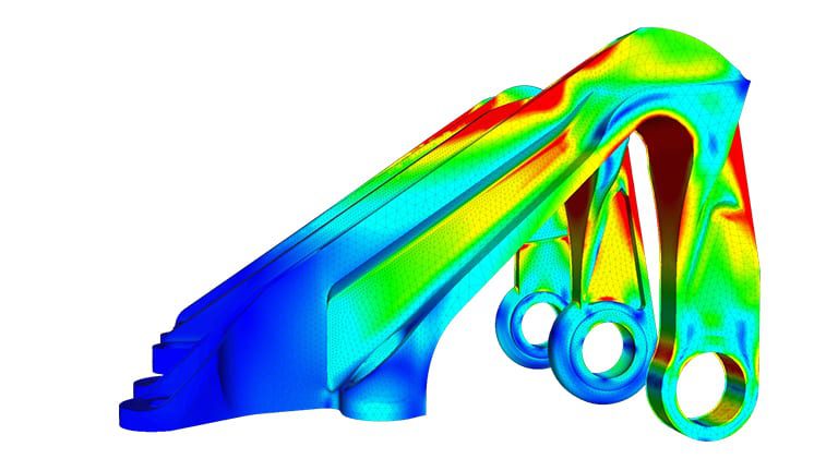
What are the Applications of the Finite Element Method?
The finite element method started with significant promise in the modeling of several mechanical applications related to aerospace and civil engineering. The applications of the finite element method are only now starting to reach their potential. One of the most exciting prospects is its application in coupled problems such as:
- Fluid-structure interaction
- Thermomechanical, thermochemical, thermo-chemo-mechanical problems
- Biomechanics
- Biomedical engineering
- Piezoelectric, ferroelectric, and electromagnetics
There have been many alternative methods proposed in recent decades, but their commercial applicability is yet to be proven. In short, FEM has just made a blip on the radar!
For more information on FEM and FEA, read our guide to FEA.
What Partial Differential Equations are in FEM?
Firstly, it is important to understand the different genres of PDEs and their suitability for use with FEM. Understanding this is particularly important to everyone, irrespective of the motivation for using finite element analysis. It is critical to remember that FEM is a tool, and any tool is only as good as its user.
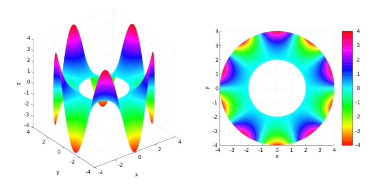
PDEs can be categorized as elliptic, hyperbolic, and parabolic. When solving these differential equations, boundary and/or initial conditions need to be provided. Based on the type of PDE, the necessary inputs can be evaluated. Examples of PDEs in each category include:
- The Poisson equation (elliptic)
- The Wave equation (hyperbolic)
- The Fourier law (parabolic)
There are two main approaches to solving elliptic PDEs, namely the finite difference methods (FDM) and variational (or energy) methods. FEM falls into the second category. Variational approaches are primarily based on the philosophy of energy minimization.
Hyperbolic PDEs are commonly associated with jumps in solutions. For example, the wave equation is a hyperbolic PDE. Owing to the existence of discontinuities (or jumps) in solutions, the original FEM technology (or Bubnov-Galerkin Method) was believed to be unsuitable for solving hyperbolic PDEs. However, over the years, modifications have been developed to extend the applicability of FEM technology.
Before concluding this discussion, it is necessary to consider the consequence of using a numerical framework that is unsuitable for the type of PDE. Such usage leads to solutions that are known as “improperly posed.” This could mean that small changes in the domain parameters lead to large oscillations in the solutions, or that the solutions exist only in a certain part of the domain or time, which are not reliable. Well-posed explications are defined as those where a unique solution exists continuously for the defined data. Hence, considering reliability, it is extremely important to obtain well-posed solutions.
For more information on PDEs in finite element analysis, see partial differential equations in FEA.
How Does FEM Work?
The principle of minimization of energy forms the primary backbone of the finite element method. In other words, when a particular boundary condition is applied to a body, this can lead to several configurations, but only one particular configuration is realistically possible or achieved. Even when the simulation is performed multiple times, the same results prevail. Why is this so?
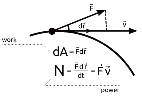
This is governed by the principle of minimization of energy, which states that when a boundary condition (like displacement or force) is applied, of the numerous possible configurations that the body can take, only that configuration where the total energy is minimum is the one that is chosen.
For more information on the variation principle (minimum potential energy), see the variation principle in FEM.
What is the History of the Finite Element Method?
Technically, depending on one’s perspective, FEM can be said to have had its origins in the work of Euler, as early as in the 16th century. However, the earliest mathematical papers on FEM can be found in the works of Schellback [1851] and Courant [1943].
FEM was independently developed by engineers to address structural mechanics problems related to aerospace and civil engineering. The developments began in the mid-1950s with the papers of Turner, Clough, Martin, and Topp [1956], Argyris [1957], and Babuska and Aziz [1972]. The books by Zienkiewicz [1971] and Strang, and Fix [1973] also laid the foundations for future development in FEM.
An interesting review of these historical developments can be found in Oden [1991].
For a review of FEM development over the last 75 years, read 75 years of FEM (a review).
What are the Most Important Technical Points to Learn in FEM?
The finite element method is in itself a semester course. In this article, a concise description of the mechanism of FEM is described. Consider a simple 1-D problem to depict the various stages involved in FEA.
Weak Form
One of the first steps in FEM is to identify the PDE associated with the physical phenomenon. The PDE (or differential form) is known as the strong form, and the integral form is known as the weak form. Consider the simple PDE shown below. The equation is multiplied by a trial function v(x) on both sides and integrated with the domain [0,1].
$$ u^{\prime\prime}(x) = f(x) $$
$$ \int {u^{\prime\prime}(x) v(x)} = \int {f(x) v(x)} $$
Now, using integration of parts, the LHS of the above equation can be reduced to:
$$ u^{\prime}(x) v(x)|_{0}^{1} – \int{u^\prime(x) v^\prime(x)} = \int{f(x) v(x)} $$
As it can be seen, the order of continuity required for the unknown function u(x) is reduced by one. The earlier differential equation required u(x) to be differentiable at least twice while the integral equation requires it to be differentiable only once. The same is true for multi-dimensional functions, but the derivatives are replaced by gradients and divergence.
Without going into the mathematics, the Riesz representation theorem can prove that there is a unique solution for u(x) for the integral and hence the differential form. In addition, if f(x) is smooth, it also ensures that u(x) is smooth.
Discretization
Once the integral or weak form has been set up, the next step is the discretization of the weak form. The integral form needs to be solved numerically and hence the integration is converted to a summation that can be calculated numerically. In addition, one of the primary goals of discretization is also to convert the integral form to a set of matrix equations that can be solved using well-known theories of matrix algebra.
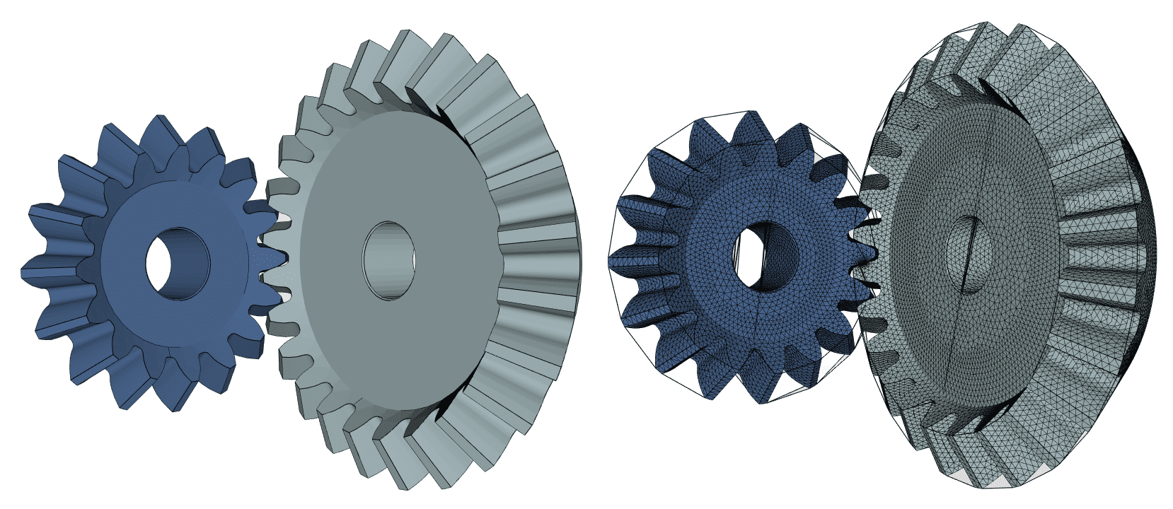
As shown in Figure 4, the domain is divided into small pieces known as “elements,” and the corner point of each element is known as a “node.” The unknown functional u(x) is calculated at the nodal points. Interpolation functions are defined for each element to interpolate for values inside the element using nodal values. These interpolation functions are also often referred to as shape or ansatz functions. Thus the unknown functional u(x) can be reduced to:
$$ u(x) = \sum_{n=1}^{nen} N_i u_i $$
where \(nen\) is the number of nodes in the element, and \(N_i\) and \(u_i\) are the interpolation function and unknowns associated with node \(i\), respectively. Similarly, interpolation can be used for the other functions v(x) and f(x) present in the weak form so that the weak form can be rewritten as
$$ \left(\sum_{n=1}^{nen} N_i u_i\right)^{\prime} \left(\sum_{n=1}^{nen} N_i v_i\right)\Bigg|_{0}^{1} – \int \left(\sum_{n=1}^{nen} N_i u_i\right)^{\prime} \left(\sum_{n=1}^{nen} N_i v_i\right)^{\prime} = \int \left(\sum_{n=1}^{nen} N_i f_i\right) \left(\sum_{n=1}^{nen} N_i v_i\right) $$
$$ \left(\sum_{n=1}^{nen} N_i^{\prime} u_i\right) \left(\sum_{n=1}^{nen} N_i v_i\right)\Bigg|_{0}^{1} – \int \left(\sum_{n=1}^{nen} N_i^{\prime} u_i\right) \left(\sum_{n=1}^{nen} N_i^{\prime} v_i\right) = \int \left(\sum_{n=1}^{nen} N_i f_i\right) \left(\sum_{n=1}^{nen} N_i v_i\right) $$
The summation schemes can be transformed into matrix products and can be rewritten as
$$ \sum_{n=1}^{nen} N_i f_i = [M]\{f\} $$
$$ \sum_{n=1}^{nen} N_i^{\prime} f_i = [M^{\prime}]\{f\} $$
The weak form can now be reduced to a matrix form [K]{u} = {f}
$$ \{v\}^T \left[ [M]^T [M^{\prime}] \right]\Big|_{0}^{1} \{u\} – \{v\}^T \left[ \int [M^{\prime}]^T [M^{\prime}] \right] \{u\} = \{v\}^T \left[ \int [M]^T [M] \{f\} \right] $$
$$ \underbrace{\left[ \left( [M]^T [M^{\prime}] \right)\Big|_{0}^{1} – \int [M^{\prime}]^T [M^{\prime}] \right]}_{[K]} \{u\} = \underbrace{\left[ \int [M]^T [M] \{f\} \right]}_{\{R\}} $$
Note above that the earlier trial function v(x) that had been multiplied does not exist anymore in the resulting matrix equation. Also, [K] is known as the stiffness matrix, {u} is the vector of nodal unknowns, and {R} is the residual vector. Further on, using numerical integration schemes, like Gauss or Newton-Cotes quadrature, the integrations in the weak form that forms the tangent stiffness and residual vector are also handled easily.
A lot of mathematics is involved in the decision of choosing interpolation functions, which requires knowledge of functional spaces (such as Hilbert and Sobolev).
For more details, read our guide How can I learn FEA? and the references listed there.
Solvers
Once the matrix equations have been established, the equations are passed on to a solver to solve the system of equations. Depending on the type of problem, direct or iterative solvers are generally used. A more detailed overview of the solvers and how they work, as well as tips on how to choose between them, are available in the blog article “How to Choose Solvers: Direct or Iterative?“
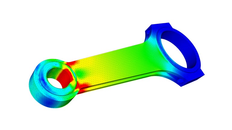
Explore FEA in SimScale
Run structural, thermal, and vibration analyses in your web browser, with no installation or special hardware.
What are the Different Types of Finite Element Method?
As discussed earlier, traditional FEM technology has demonstrated shortcomings in modeling problems related to fluid mechanics and wave propagation. Several improvements have been made recently to improve the solution process and extend the applicability of finite element analysis to a wide range of problems. Some of the important ones still being used include:
Extended Finite Element Method (XFEM)
Bubnov-Galerkin method requires continuity of displacement across elements. Although problems like contact, fracture, and damage involve discontinuities and jumps that cannot be directly handled by the finite element method. To overcome this shortcoming, XFEM was born in the 1990’s. XFEM works through the expansion of the shape functions with Heaviside step functions. Extra degrees of freedom are assigned to the nodes around the point of discontinuity so that the jumps can be considered.
Generalized Finite Element Method (GFEM)
GFEM was introduced around the same time as XFEM in the 90’s. It combines the features of the traditional FEM and meshless methods. Shape functions are primarily defined by the global coordinates and further multiplied by partition-of-unity to create local elemental shape functions. One of the advantages of GFEM is the prevention of re-meshing around singularities.
Mixed Finite Element Method
In several problems, like contact or incompressibility, constraints are imposed using Lagrange multipliers. These extra degrees of freedom arising from Lagrange multipliers are solved independently. The system of equations is solved like a coupled system of equations.
hp-Finite Element Method
hp-FEM is a combination of automatic mesh refinement (h-refinement) and an increase in the order of polynomial (p-refinement). This is not the same as doing h- and p- refinements separately. When automatic hp-refinement is used, and an element is divided into smaller elements (h-refinement), each element can have different polynomial orders as well.
Discontinuous Galerkin Finite Element Method (DG-FEM)
DG-FEM has shown significant promise for utilizing the idea of finite elements to solve hyperbolic equations, where traditional finite element methods have been weak. In addition, it has also shown improvements in bending and incompressible problems which are typically observed in most material processes. Here, additional constraints are added to the weak form that includes a penalty parameter (to prevent interpenetration) and terms for other equilibrium of stresses between the elements.
Going Beyond Linear: Nonlinear FEA
While the finite element method often assumes linear material behavior, many real-world applications require nonlinear material models — from metals yielding under overload to rubber seals stretching 300%. Understanding when and how to go nonlinear is a critical skill for practicing engineers.
Frequently Asked Questions
The finite element method (FEM) is a numerical technique for solving the partial differential equations that describe physical behavior. It divides the domain into small elements, approximates the solution on each element with simple interpolation functions, and assembles the results into a system of algebraic equations that a computer solves.
FEM is the mathematical method. FEA is the application of that method to analyze a specific part or system, for example the stress in a bracket or the temperature in a heat sink. Engineers run FEA in simulation software, and the software uses FEM to compute the result.
In engineering, FEM stands for finite element method. The related term FEA stands for finite element analysis.
FEM is used for structural analysis (stress, deformation, buckling), vibration and modal analysis, heat transfer, thermomechanical problems, fluid-structure interaction, biomechanics, and electromagnetics. Engineers use it to check designs against loads and failure criteria before building physical prototypes.
FEM converts the governing partial differential equation into its weak (integral) form, divides the domain into a mesh of elements, and approximates the unknown field on each element with interpolation functions defined at the nodes. This produces a matrix equation [K]{u} = {f}, which a solver computes for the unknown nodal values.
FEM Conclusion
We hope this article has covered the answers to your most important questions regarding the finite element method. If you’d like to see it in practice, SimScale offers the possibility to carry out finite element analyses in the web browser. To discover all the features provided by the SimScale cloud-based simulation platform, download this overview or watch the recording of one of our webinars.
Materials for getting started with SimScale can be found in the blog article “9 Learning Resources to Get You Started with Engineering Simulation“.
Start simulating with SimScale
Set up your own cloud-native simulation via the web in minutes by creating an account on the SimScale platform. No installation, special hardware, or credit card is required.
References
- Schnellback, Probleme der Variationsrechnung, Journal für die reine und Angewandte Mathematik , v. 41, pp. 293-363 (1851)
- R. Courant, Variational methods for the solution of problems of equilibrium and vibrations, Bulletin of American Mathematical Society, v. 49, pp. 1-23 (1943)
- M. J. Turner, R. M. Clough, H. C. Martin and L. J. Topp, Stiffness and deflection analysis of complex structures, Journal of Aeronautical Science, v. 23, pp. 805-823 (1956)
- J. H. Argyris, Die matritzentheorie der Statik, Ingenieur-Archiv XXV, pp. 174-194 (1957)
- O. C. Zienkiewicz, The Finite Element Method in Structural and Continuum Mechanics, McGraw-Hill, London (1971)
- I. Babuska and A. K. Aziz, Survey lectures on the mathematical foundations of the finite element method, In The Mathematical Foundation of the Finite Element Method with Applications to Partial Differential Equations, pp. 3-636 (1972)
- G. Strang and G. J. Fix, An analysis of the Finite Element Method, Prentice-Hall, Englewood Cliffs, New Jersey (1973)
- J. T. Oden, Finite elements: An introduction, in Handbook of Numerical Analysis II, Finite element methods (Part I), North-Holland, Amsterdam, pp. 3-12 (1991)