In this article, we explore the black box of numerics and the task of choosing a FEM solver. In general, there are a typical set of options that work for a FEM problem and we never change it. These are like those magic parameters that we never change, and we often do not even know why they are assigned those values. This time, we open the black box to see what they mean and how they affect the solution.
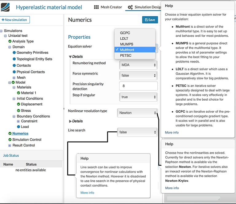
As shown in Fig. 01, we can see that, for structural mechanics simulations, there are several options available in the numerics section of the SimScale cloud-based platform. Of these, Multfront, MUMPS, and LDLT are direct solvers, while PETSc and GCPC are iterative solvers. In addition, there are other options called “Nonlinear resolution type” and “Line search” features. What do all of these mean?
FEM Solver Direct Solver or Iterative Solver: What is the Difference?
When we use the finite element method (FEM), we are solving a set of matrix equations of the form [K]{u} = {f}. Here [K] is referred to as the stiffness matrix; {f} as the force vector and {u} as the set of unknowns. There are several methods available that can directly solve this system of equations. A simple and direct way—though not recommended—would be to invert the matrix [K] and multiply with force vector {f}. This results in solutions to the unknowns. However, an inverse is almost never calculated. More commonly adopted approaches to directly calculate the solution include Gaussian elimination, LU, Cholesky, and QR decompositions.
However, such direct methods fail when the matrices are:
- Very large, for example, in the order of a few million: If the matrix is of order n, then n x n x n operations are needed to solve the system using Gaussian elimination. Imagine that the system has 10 million unknowns; in this case, it would need operations of the order of ExaFlops.
- Have a lot of zeros (often referred to as sparse matrices): Sparse matrices have a lot of zeros in the matrix. Operating upon them (like multiply zero by zero) is both a waste of computing resources and completely meaningless.
- Do not have direct access to the entire matrix at once
In contrast to the direct solver, the iterative solver starts by assuming an approximate solution for the unknowns {u}. The solution is iterated upon to reach an “exact” solution.
The purpose of a helmet is to protect the person who wears it from a head injury during impact. In this project, the impact of a human skull with and without a helmet was simulated with a nonlinear dynamic analysis. Download this case study for free.

FEM Solver What is a Sparse Matrix?
Sparse matrices are commonly encountered in finite element analysis. As seen above, FEM involves a lot of matrix operations. In order to save both time and storage space, a sparse matrix is preferred.
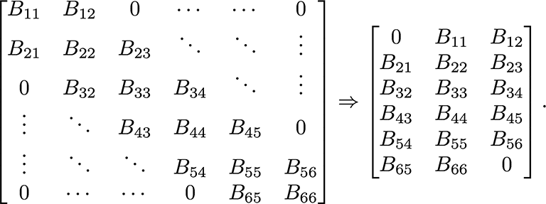
As shown in Fig. 02, the matrix on the LHS, where all non-zero numbers are on either side of the diagonal and zeros are far away, are commonly known as banded matrices. Such a matrix has a lot of zeros. This matrix is compressed and stored in a format where the zeros are dropped. Such a matrix is called a sparse matrix.
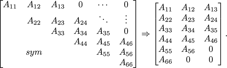
As shown in Fig. 03, the advantage is even greater when a symmetric matrix is being stored in a “sparse” format. In this case, only half of the matrix is stored. As illustrated, the number of non-zero quantities are much higher in the A-matrix in Fig. 03. However, it is clear that the total space taken is the same as B-matrix in Fig. 02. Instead of 36 places, only 18 places are being used. Imagine the savings if this matrix was over a million times a million in size!
Iterative Solver How Does an Iterative Solver Actually Work?
Just as earlier discussed, let us imagine we are solving the equation [K]{u} = {f}. Then an approximate initial guess {u0} is made. Using this {u1} is calculated and then again {u2} and so on. The procedure is continued until we reach a solution {un} such that [K]{un}-{f} is almost zero. Remember that the computer cannot reach an exact zero when using real numbers!
To give an elaborate answer, a simpler matrix [A] is chosen to start with. A general choice is [A] = diag[K]. Only the diagonal elements of [K] are taken in [A] to start with. Using this matrix [A], {u1} is calculated from {u0} by directly solving the equation.

Iterating for n-steps, the equation becomes

This continues until {u}, which satisfies that the original equation is found.
In addition, an iterative solver uses a procedure called “preconditioning”. In the simplest terms, the condition number of a matrix can be expressed as the ratio of the absolute value of biggest to smallest number in the matrix. As the condition number increases, the equation system becomes less stable.
When an iterative solver is used, a preconditioning procedure is done before starting the solution process. This improves the condition number of the matrix. Consider the above system [K]{u} = {f}. Now multiply by a matrix [M], then we have [M][K]{u} = [M]{f}. This does not change the solution {u} but depending on the properties of the matrix [M], it can change the overall behavior of the system.
Direct Solver Direct Solver: What Are the Options? How to Choose Among Them?
SimScale supports three direct solvers for structural mechanics problems: LDLT, Multfront, and MUMPS. LDLT and Multfront offer nearly the same options and will be discussed first. Following this, MUMPS and its options will be discussed. A general rule of thumb to choosing direct solvers is based on the number of degrees of freedom in the system.
Calculating the Number of Degrees of Freedom of a System
Let us say that we are solving a FEM problem in 3D and the mesh has n-nodes. For a purely mechanical problem, we are solving for three unknowns at each node. These are the displacements along x-, y-, and z-directions. Therefore, the total degrees of freedom is given by:

For a more general case, like thermo-mechanical or electro-hydro-thermo-mechanical problems, where:
- number of dimensions = d
- number of unknowns at each node = p
- number of nodes in the mesh = n
The total degrees of freedom of the system is given as:

Choosing Options for LDLT and Multfront
In general, the default options should work well. However, it could be useful to know what the numbers mean.
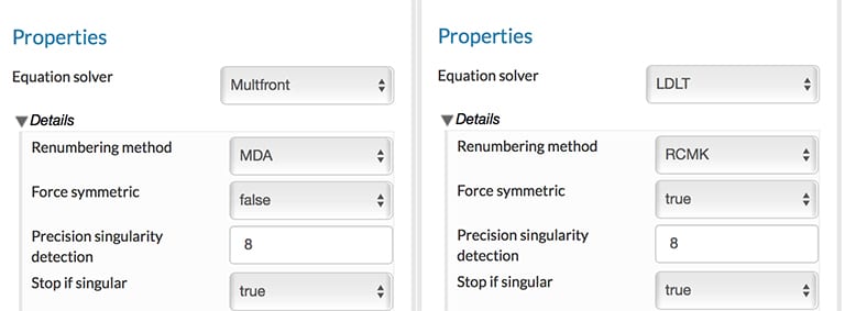
The options for these solvers are as shown in Fig. 04. The first option is the “renumbering method”. Going back to the start of this article, we examined the sparse matrix and bandwidth. This option optimizes the node numbers so that the bandwidth of the matrix is as small as possible. SimScale uses different algorithms for optimization based on the solver used. It is strongly advised to use this option. For the LDLT solver, RCMK is the only option. Alternatively, for the Multfront solver, use MD for smaller problems with up to 50,000 degrees of freedom and use MDA for larger problems.
The second option is regarding “force symmetric”. Again, if we remember Fig. 03, it was demonstrated that only half the matrix was stored if the matrix was symmetric. “True” could be chosen if one is certain that the matrices are symmetric in nature. This can significantly save on both memory and time. For example, problems using linear elastic or hyperelastic material and no inelastic effects result in symmetric matrices. If one is unsure, using “False” could be a safer option.
The last option concerns the determinant of the stiffness matrix. This is generally used more often in normalizing during the solution process, and it is also related to the stability and uniqueness of the solution. If the determinant is used to normalize, it will be used in the denominator of a fraction. Thus, if it is very small, the fraction can increase rapidly leading to instability. The option sets to stop the simulation if the determinant is very small of the order of 10^- (Precision singularity detection). Always remember that the computer never reaches an exact zero! It is recommended to keep this option as “True”.
Additional Options for MUMPS
MUltifrontal Massively Parallel Sparse direct solver (or MUMPS) is a sparse solver that is optimized for solving the system of equations in parallel. It offers additional options for customization of parallel computing. For general use, the default options are recommended.
Alongside the above-discussed options, some alternatives that may be of interest to advanced FEM simulation users would be:
- Renumbering scheme – SCOTCH and PARD methods are quite superior. The automatic option is recommended if one is unaware of these schemes.
- Single precision – It is strongly advised to use “False”. Using single precision could lead to faster computations, but it could also lead to convergence problems for nonlinear problems.
- Distributed matrix storage – “True” is recommended if one uses multiple processors for the computation. This will take advantage of parallel computing to save the results
- Matrix type – This sets the type of matrix: if symmetric, etc. The “automatic” option is the best to use unless one is completely sure.
Which of the Three Direct Solvers to Use?
If the size of the FEM problem is small, say about 50,000 degrees of freedom, LDLT is a simple and easy to use solver. For larger problems, Multfront is recommended. For advanced users and those who intend to use parallel computing to the best, MUMPS is the best option available.
FEM Solvers Iterative Solver: What Are the Options? How to Choose Among Them?
SimScale supports two iterative solvers for structural or FEM problems: PETSc and GCPC.
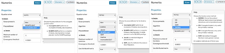
Both PETSc and GCPC solvers use pre-conditioning and allow different options. As evident from Fig. 05, the options in GCPC are much more limited and also offered by PETSc. A general rule of thumb when choosing between the two is that GCPC is good for beginner users who are running smaller problems, whereas PETSc is more suited for advanced users who are running larger problems and are interested in customizing.
There are two main options that need to be considered here: pre-conditioning technique and solution algorithm. As discussed earlier, pre-conditioning technique improves the condition number of the matrix. The solution algorithm is what does the actual work of solving the system of equations.
There are several preconditioners available, and it is recommended to explore them to find a solution that works for your exact needs. There is no “fits all” solution here. In general, MUMPS LDLT is a recommended option as it takes advantage of the MUMPS package. Personally, SOR is my favorite since it offers stability for problems involving nonlinear elasticity.
With regard to the solvers, GCPC is limited to CG solver. PETSc offers several other options. CG (Conjugate Gradient) and CR (Conjugate Residual) work only for symmetric matrices, while GCR (Generalized Conjugate Residual) treats all matrices. GMRES is my favorite. GMRES provides a great balance between computational speed, robustness, and reliability. If you are unsure, GMRES is always a safe bet.
Solver Options
The “nonlinear resolution” option provides more customization options for the user. At each global iteration (of direct solver) or local + global iteration (of iterative solver), a simple algorithm is used to solve the equations. Here simple algorithms like Newton-Raphson, quasi-Newton, etc. are used. For the direct solvers, only the “Newton” option is available. “Newton-Krylov” is optimized for iterative solvers and strongly recommended.
Firstly, it is a good practice to use the same option for both the “prediction matrix” and “Jacobian matrix” options. Using the “tangent matrix” calls the Newton method, while “elastic matrix” calls a quasi-Newton method. The quasi-Newton method is recommended for coupled problems where the matrices might not have all the nice properties. For example, in a thermomechanical problem, the quasi-Newton method is well suited. Otherwise, the Jacobian option (or full Newton method) is strongly recommended for accurate solutions to structural problems.
If the problem is well-posed, the Newton method demonstrates “quadratic convergence.” This means that convergence is reached in 3-7 iterations. In several scenarios, this might not always happen. One of the most common reasons is that the chosen time step is too large for that part of the problem. In this case, the problem will not reach convergence. If an automatic time stepping is chosen, then the time step size is reduced until convergence is reached. The maximum number of iterations when the system declares a non-convergence and reduces the time step can be selected here. The default value of 15 is generally sufficient.
Line Search Is Line Search Necessary? When Should It Be Used?
Line search reduces the calculated step size into much smaller increments. Since the step sizes are smaller, this automatically improves convergence. Line search is not always necessary, even in the presence of nonlinearities. However, it is recommended in elastoplastic problems that involve yielding of materials. Here the derivative of the stiffness matrix is rapidly changing at the yield point. Line search can significantly improve the convergence in such scenarios. However, the line search is discouraged in the presence of contact constraints.
For a purely elastic problem, a line search is generally not necessary.
FEM Solver Summarizing FEM Solvers
- Direct solver or iterative solver?
- Direct solver if the number of degrees of freedom is less than one million
- Which direct solver to use?
- If the number of degrees of freedom is less than 50,000, LDLT works well
- For larger problems, Multfront is advised
- To use the full potential of parallel computing, use MUMPS
- Which iterative solver to use?
- PETSc and GMRES are my favorites
- For smaller problems, the GCPC iterative solver is also worth a try
- Setting Nonlinear resolution options
- For direct solver, use the “Newton” option and “Newton-Krylov” for an iterative solver
- For prediction and Jacobian matrix, use “tangent matrix” for structural problems and “elastic matrix” for coupled problems
- When to use line search?
- Useful for elastoplastic problems involving yielding of materials.
I hope this article has covered the answers to your most important questions regarding FEM solvers and how to choose between them for a simulation. If you’d like to put the theory into practice, SimScale offers the possibility to carry out finite element analyses in the web browser. Just create a free Community account here to try it out.
Additionally, watch the recording of our “More Durable Consumer Products with FEA” webinar. All you need to do is fill out this short form and it will play automatically.