How to Run a Non-Linear Rubber Simulation: Bidirectional Sealing System Walkthrough

You already know rubber breaks linear FEA in three ways at once: large strain, near-incompressibility, and frictional contact. What you probably don’t want to hear is that most first-time non-linear runs of a sealing system diverge inside ten minutes, usually because the contacts close badly, the hyperelastic parameters were copied from a textbook, or the result controls were never set. This walkthrough fixes all three.

By the end of it, you’ll have set up a non-linear rubber simulation of a bidirectional rod seal, end to end, using the Hexagon Marc solver inside SimScale. Eight steps. Browser-based. No installation, no licence pool. The output you’ll walk away with: contact pressure along the seal, plastic deformation regions, and the actuator load on the rod, all from a single multi-step run.

Why Non-Linear Is Non-Negotiable for Rubber

Three things happen to rubber at the same time, and a linear analysis cannot represent any of them:

• Large deformation. Rubber routinely strains 30–300%. Stiffness depends on the deformed shape, which itself depends on the load — geometric nonlinearity is mandatory.
• Hyperelastic, near-incompressible material. The stress-strain response is non-linear, the bulk modulus is orders of magnitude higher than the shear modulus, and Young’s modulus is meaningless. You need a calibrated hyperelastic material model — Mooney-Rivlin, Ogden, Yeoh, or Marlow — driven by real test data.
• Contact and friction. Seals work because of contact. Surfaces touch, separate, and slide, with pressure-dependent friction. Contact is inherently non-linear and is usually the dominant source of solver pain.

Plastic components (D-shape rings, anti-extrusion rings) add a fourth: elastoplasticity, with permanent deformation possible after a single pressure cycle.

A successful non-linear rubber simulation has to handle all of these in the same model, across a load history that mirrors the real-world assembly and pressurization sequence. That’s exactly what the bidirectional rod seal example below does.

Model and Parameters

The example is a 1° axisymmetric sector of a bidirectional rod seal: the kind of model that ships hydraulic and pneumatic components every day:

Component	Material class	Role
Rod	Steel	Translates up and down, transfers load
Groove	Steel	Fixed housing
D-shaped seal	Plastic (elastoplastic)	Sealing Element
Quad-ring	Rubber (hyperelastic)	Energizing element
Tool	Steel	Auxiliary part used to position the quad-ring during assembly

The 1° sector cuts compute cost by two orders of magnitude versus a full revolution, while preserving accuracy through symmetry boundary conditions on the two cut planes.

The job is split into four load steps that reproduce the physical sequence:

1. The tool pushes the quad-ring into the groove.
2. The tool retracts.
3. 50 bar pressurizes from the top.
4. 50 bar pressurizes from the bottom.

Steps 3 and 4 test the seal in both flow directions — that’s what makes it bidirectional, and that’s what determines whether the part actually ships.

How to Set Up the Simulation

The setup follows SimScale’s top-to-bottom tree. Work through each item until every section shows a green checkmark. Everything from CAD import to post-processing happens in the same browser-based workbench.

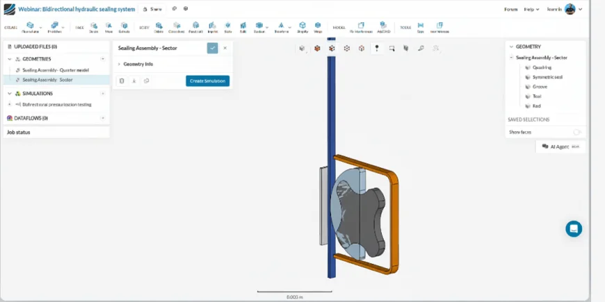
Step 1: Upload Your Geometry and Use Symmetry

Drag your CAD file onto the SimScale workspace. STEP, IGES, X_T, and native CAD formats (SolidWorks, Inventor, Creo, CATIA) all upload directly. For axisymmetric or rotationally repeating geometry, cut a thin sector, a 1° wedge, to slash mesh size and runtime. Make sure your cut planes are clean and that all five parts (rod, groove, D-seal, quad-ring, tool) are present in the sector.

Step 2: Create a Nonlinear Mechanical Simulation

Hit Create simulation and choose the Nonlinear Mechanical analysis type. This routes your job to the Hexagon Marc solver, which is built for large deformation, complex contact, and hyperelastic materials. CFD, electromagnetics, and linear structural analyses live in the same workspace, so the same CAD can be reused for coupled studies later.

Step 3: Define Contacts Between Components

Contact is the heart of a sealing simulation, and you’ll define six contact pairs covering every interface that can come together during the four load steps. SimScale supports two types:

• Touching contact (no penetration, can separate) — your default for rubber-on-metal.
• Bonded contact (tied) — for permanently joined parts.

Add friction where it matters (rod–quad-ring, rod–D-seal). Use the load-step controls to activate or deactivate specific contacts in different steps — for example, the tool–quad-ring contact is only active during the assembly steps, and you remove it once the tool retracts. If your assembly has dozens of interfaces, Automatic Contact Detection configures them in one click.

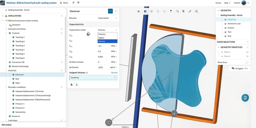
Step 4: Assign Hyperelastic and Elastoplastic Materials

Material assignment is the second-largest source of error in non-linear rubber FEA. (The largest is forgetting to define result controls. We’ll get to that.)

• Quad-ring (rubber). Choose hyperelastic. Mooney-Rivlin handles moderate strain (<100%) when you have limited test data. Ogden handles strains beyond 100% if you have shear and biaxial data. Yeoh is a safe single-parameter option when only uniaxial data exists. Marlow, available on the Marc backend, fits any uniaxial test curve directly without parameter tuning — Hexagon specifically calls it out for “accurately predicting the behavior of rubber seals and soft tissues.” Whatever you pick, calibrate against tests that match the loading state, not just one uniaxial curve. SimScale ships validated hyperelastic test cases for uniaxial, equibiaxial, and planar tension you can use as benchmarks. Full input syntax is in the hyperelastic materials documentation.
• D-shaped seal (elastoplastic). Use elastoplastic with isotropic hardening. A linear-elastic law will badly under-predict deformation once the seal yields under pressure.
• Rod, groove, tool (steel). Standard linear-elastic steel. These parts barely deform — using a richer model wastes compute.

Step 5: Apply Boundary Conditions and Multi-Step Loading

Boundary conditions drive the physics. For the bidirectional seal:

• Groove: fully fixed for all four load steps.
• Tool: prescribed displacement via a tabular input — push down in step 1, retract in step 2, then zero for steps 3 and 4.
• Rod: prescribed displacement via a separate table — moves up in step 3, down in step 4. Or fully constrained, depending on your test case.
• Pressure: 50 bar on the top exposed face during step 3; 50 bar on the bottom face during step 4. Steps 1 and 2 stay pressure-free so the seal can be assembled before any fluid load is applied.
• Symmetry: two symmetry planes constrain the 1° sector. Assign every part to both planes — miss this and the geometry will fly apart.

The tabular input is what makes the multi-step setup clean: a single boundary condition follows a custom load history without you having to split it into separate definitions per step.

Step 6: Configure Load Steps and Solution Control

In Solution control, set total simulation time to 4 seconds (one second per load step) and start with a small initial increment, around 0.01 s, so the solver can capture contact closure and the onset of plastic flow without bisecting endlessly. Turn on adaptive time stepping. Allocate cores based on model size — four cores handle this case comfortably; the platform scales to 192 cores for full-revolution or fine-mesh jobs.

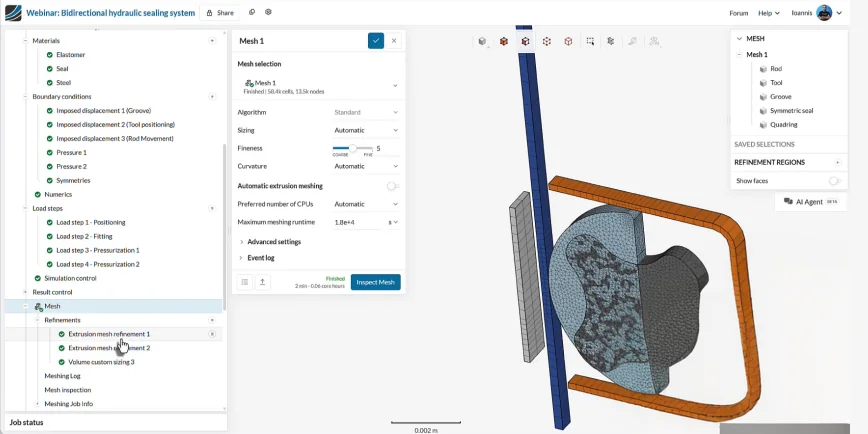
Step 7: Mesh the Model with Marc Technology

Use a coarser tetrahedral mesh on the rod, groove, and tool (rigid-body-like behavior) and a finer mesh on the quad-ring and D-seal where strain gradients are steep. Marc’s tet element formulation is robust against the mesh distortion that breaks lesser solvers when rubber compresses 50% or more.

Two practical rules:

• Resolve at least three to four elements through the seal cross-section in the contact zone.
• Avoid sliver elements at sharp seal corners — they cause Jacobian failures during compression.

Step 8: Set Result Controls Before You Run

This is the step engineers skip and then regret. Result controls must be defined before you submit the run, or those quantities won’t be written, full stop. Add at minimum:

• Contact pressure — the primary KPI for any seal.
• Equivalent plastic strain — flags any permanent deformation in the D-seal.
• Contact body force — total force on the rod (or any selected part), used to validate against analytical seal-force estimates.

Hit Start. The job launches in the cloud, you get an email when it’s done, and you don’t have to keep your laptop awake.

Results: Contact Pressure, Plastic Strain, and Contact Body Force

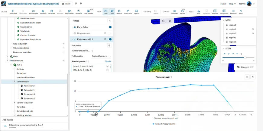
Post-processing answers three questions, in order, that determine whether the seal works.

1. Does the seal hold? Plot contact pressure between the rod and the quad-ring at the end of step 3 (top pressurization) and step 4 (bottom pressurization). Use the plot-over-path tool to extract the pressure profile along the contact line.

Takeaway: minimum contact pressure must exceed the upstream fluid pressure (50 bar here) plus a safety margin. If it drops below, the seal leaks — design change required.

2. Is the seal damaged? Inspect equivalent plastic strain on the D-shaped sealant. Localized plastic strain above ~2% means permanent deformation — the seal won’t return to its original shape after depressurization, and seal performance degrades cycle by cycle.

Takeaway: in the example case, a high-plastic-strain region appears at the corner of the D-seal. That’s a redesign signal, not a “ship it” signal.

3. What load does the seal place on the rod? The contact body force result control gives the total force the rubber exerts on the rod at every time step. This output feeds directly into actuator sizing, hydraulic pressure rating, and friction-loss estimates.

Move the time slider to inspect intermediate states: assembly distortion, contact closure, max von Mises stress location, and any region where the quad-ring is being squeezed beyond its elastic limit.

Where Non-Linear Rubber Simulations Pay Off

The same workflow scales to any rubber component where contact and large strain matter:

• Hydraulic and pneumatic seals — rod seals, piston seals, rotary seals. Marc is used routinely for “critical sealing analyses in the oil and gas sector.”
• O-rings and gaskets — including the famous Challenger O-ring failure that motivated decades of seal-simulation R&D.
• Vibration isolators and engine mounts — large compressive strain, frequency-dependent response.
• Tire components — tread, sidewall, bead, treadwear.
• Elastomeric bearing pads — see SimScale’s bridge bearing pad case study.
• Medical device seals — syringe plungers, valve membranes, stent crimping.
• Snap-fit assemblies — see the snap-fit assembly tutorial for a related plastic-deformation walkthrough.

The pattern is identical across all of them: hyperelastic material, contact pairs, multi-step load, symmetry where applicable.

Common Pitfalls in Non-Linear Rubber FEA

Most failed runs come down to five recurring issues:

• Convergence failure during contact closure. Reduce the initial time step, use stiffness-proportional damping, or apply contact gradually with a soft-touch. SimScale’s KB has a dedicated troubleshooting guide for parts colliding in non-linear runs.
• Volumetric locking with fully integrated tet elements on near-incompressible rubber. Use the Marc-recommended hybrid formulation for hyperelastic regions.
• Mesh distortion in highly compressed regions. Pre-distort the mesh in the loaded direction or use a remesher for very large deformation.
• Wrong material parameters. Mooney-Rivlin coefficients calibrated on uniaxial data alone will under-predict biaxial response. Always include test modes that match the loading state.
• Forgetting to define result controls. There’s no way to recover contact pressure or plastic strain from a run that didn’t request them.

For a deeper checklist, Modeling Elastomers Using FEM: Do’s and Don’ts is the companion read. If you’re not yet sure whether your problem even needs non-linear FEA, check When do I need a non-linear static analysis? first.

Support and Collaboration

You’re not setting this up alone. SimScale’s Engineering AI co-pilot guides you through the setup, validates your inputs, and applies organizational best practices automatically — it scales the knowledge of a senior simulation engineer across your team. Live in-product support and a community of 800,000+ engineers back you up at every stage.

For team workflows, share any project with a colleague regardless of where they are. No data download, no upload. Grant view, copy, or edit access from inside the platform.

---