Here at SimScale, there are countless ways to simulate and evaluate your designs. From CFD to FEA and thermodynamics, the possibilities are vast. But with so many possibilities, how do you always know that you are getting the most out of your simulations? In this article, we will present a simulation project from our public library that can be copied and run autonomously and provide some best practice tips including setup and guidelines to follow for conjugate heat transfer simulation.
What Is Conjugate Heat Transfer?
Conjugate heat transfer is a type of heat transfer analysis between solids and fluid(s). This type of heat transfer includes both convection (between fluids) and conductive (between solids) heat transfer, as well as both forced and natural convection. The Nusselt number can be used to validate the convective heat transfer results from such simulations. Common applications and use cases of this thermal simulation type include electronics cooling, heat exchangers, industrial machinery, some AEC cases, and more. In order to demonstrate best practices for this application type, an electronics cooling application will be used as an example.
Learn the three basic heat transfer modes in our Thermal Analysis Workshop. Watch the recording now!

Our Case: Conjugate Heat Transfer
Our project focuses on electronics cooling performance, as the CHT simulation type is most commonly used for this type of application. We will explain how to set up the analysis on the SimScale platform, what guidelines to follow to guarantee success, how to make sure your results are good, and how to make sure your solution is fully converged.
Simulation Setup
In order to provide the best practices, we will explain how to set up your simulation step by step following this project.
Step One: CAD Cleanup and Upload
Every simulation starts with a design. When it comes to electronics, “Ready-to-Manufacture” CAD models can be incredibly intricate and feature every component within the system (as pictured below). If this is the case for you, some CAD cleanup may be helpful and required because these details can unnecessarily add complexity to your model.
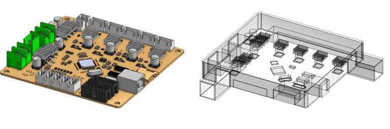
To do this, keep in mind that large sections of electronics packages have little influence over thermal performance, including bus plugs, pin connectors, etc. These sections can be simplified, and rows of buses can be approximated as a block. Next, all chip pins, numbering imprints, serial numbers, and fillets should be removed. Additionally, small bodies which are not emitting heat as well as small fillets on heat sinks, capacitors, etc., should be removed. Finally, inlet/outlet extensions should be added to help with ascertaining convergence.
Once these steps are completed, you can easily drag & drop your CAD file to the ‘Geometry Upload’ function on SimScale, or directly import via Onshape which eliminates the need to create a local file.
Step Two: Geometry Operations
After your clean CAD is uploaded, you will then have to select Geometry Operations. It is critical that every CHT simulation has a solid CAD body that represents the fluid volume. A common mistake is failing to do this, which results in assigning boundary conditions to solids instead of fluids (which is bad!). It is important that you extract the fluid volume. For more information, watch the video below.
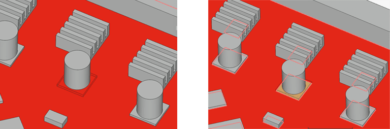
To do this, go to ‘add geometry operation’, select ‘open inner region’ (meaning we will select faces surrounding openings of our solid casings and ducts), and then select the Boundary faces and Seed face. The Boundary faces define the inlet/outlet region, and the Seed face defines a face that touches the fluid. Next, add an Imprint geometry operation. Imprinting your geometry is critical because it splits the surfaces of multiple touching bodies and generates more surfaces. This is important in order to accurately capture heat transfer between solids in a CHT simulation. In order to visualize the imprint geometry operation, see the before and after image below.
Once this is complete, you can create a new conjugate heat transfer simulation and move on to material assignments.
Step Three: Material Assignments
The best way to assign materials in electronic CAD models is to start with the items on the outside and work inwards. With this particular case, the chassis and inlet and outlet extensions are assigned as aluminum (as it is a very high thermal conductor). In the SimScale platform, we have a default material database that you can use and you can change their default material properties like the thermal conductivity, density, or specific heat.
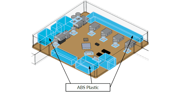
ABS plastic is assigned next. This is assigned to components such as electrical connectors and snaps. You’ll notice these components are mostly simplified blocks, and to save mesh you can even simplify a row of simplified blocks into a single CAD body (as shown in the image below). There is a significantly low thermal impact with these components, so keep in mind that their flow obstruction is the primary factor in the system’s thermal performance.
The next material assignment for this project is copper. This material is a very high thermal conductor, therefore in our case, we used the default copper from the SimScale platform and assigned all the heat sinks as this. This is a very common choice for heat sinks within an electronic system. Learn more about heat sink design and simulation. Next, silicon is selected for all capacitors and chips (underneath the heatsinks) from the SimScale database.
Finally, the last material assignment is the printed circuit board (PCB). A typical printed circuit board is made up of layers of plastic (typically FR4), with copper layers in between. This component is unique as it is not a single type of material, but for simulation purposes, it is treated as such. PCB is characterized by anisotropic thermal conductivity properties, so it is very important to take this into account for calculations. The in-plane thermal conductivity is usually very high and around 20 W/m-K, but the through-plane is usually below 1 W/m-K. To define the bulk thermal conductivity for through-plane, sum the thermal conductivities for each copper and plastic layer. This is analogous to calculating the total resistance of a set of resistors in series in an electrical circuit. Next, calculate the in-plane thermal conductivity by treating each layer as parallel to one another. This is analogous to calculating the total resistance of a set of resistors in parallel in an electrical circuit. Check out this paper for more information.
Step Four: Boundary Conditions
After all materials are assigned, boundary conditions can be set. Flow boundary conditions simply indicate to the solver what occurs at the boundaries of the system. In order to do this, the inlet and outlet faces need to be defined in terms of velocity, temperature, and pressure. For the inlet, assign a flow velocity, as well as a temperature of the flow coming in. For most simulations where the flow velocity is defined at the inlet, the outlet face should be set as 0 pressure gauge. The solver can then calculate the resulting velocity profile and temperature.
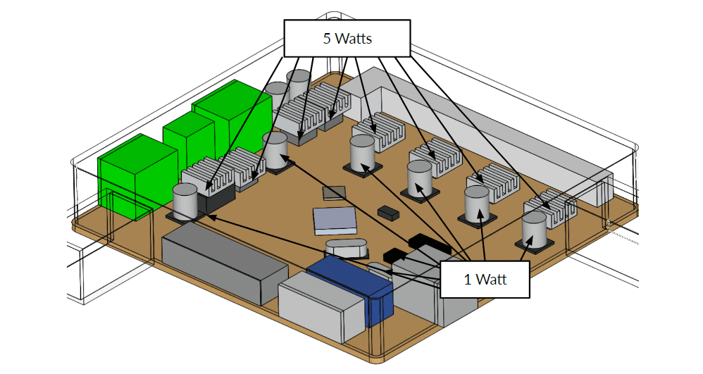
Lastly, thermal load boundary conditions are set for all the chips and capacitors within the system. For this case, we set chips at 5W and capacitors at 1W (as shown above). In SimScale, the heat load assignments to volumes are in the ‘Advanced Concepts’ section of the tree, and called ‘Power Source’. If you are having trouble finding this, watch the video provided at the bottom of this article and jump to ‘Demonstration’.
Step Five: Result Control
With steps one through four completed, the model is almost ready for a CHT simulation. The final step to judge convergence, which is particularly important for such simulations, is to set up some result control items. To do this, select some surfaces of interest (namely the inlet, outlet, heat-emitting bodies, etc.) so that you can monitor the field data (velocity, pressure, temperature, etc.) at these locations as the run progresses. This way, you can plot data over solver iterations to determine whether or not the solution has converged. A solution is considered converged when, even though you are adding more iterations, you still get the same result quantities. In other words, your simulation can be considered converged when values such as velocity, pressure, and temperature in the areas of interest stop fluctuating.
Simulation Results
The results from the CHT simulation run can be visualized above, where vector comets show the flow path of fluid through the domain. You can also see an area of fluid recirculation in the far back corner, that potentially indicates a warm section of the model. The bottom center area of the model has low airflow, as well as shows no sign of large heat loads. Consequently, the center of the domain may be a ‘dead zone’ due to the air swirl.
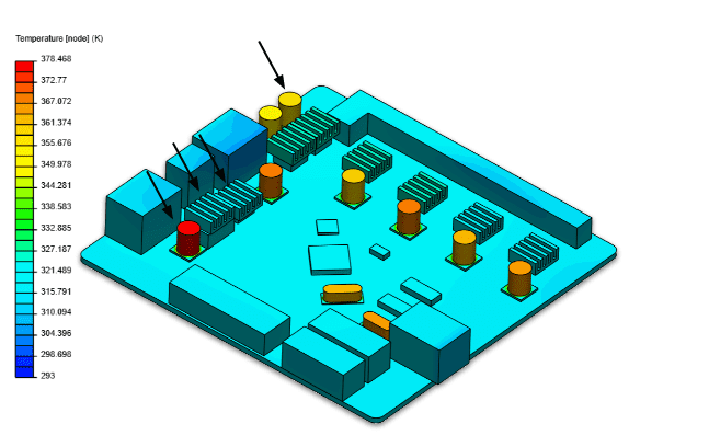
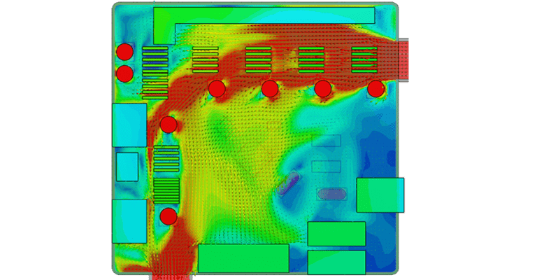
In the above image, you can see the temperature plotted globally on the model. The capacitors can be identified as the warmest components, and you can also note that some heat sinks are not aligned with the fluid flow direction.
Conjugate Heat Transfer Simulation: Conclusion
Several critical steps go into generating a successful conjugate heat transfer analysis. Preparing the CAD and de-featuring/removing unnecessary details will maximize the chances of a successful CHT analysis. Proper material definition and boundary condition pairing will ensure the physics are defined properly and let the solver do the rest. Lastly, as a simulation user, it is important to probe areas of interest and monitor convergence in order to know the results you get can be trusted.
Watch the whole step-by-step webinar here, only from SimScale.
More Conjugate Heat Transfer Resources From SimScale
- CHT Analysis
- Queuing Simulations & Auto-contacts for Conjugate Heat Transfer
- Conjugate Heat Transfer Analysis on a Raspberry Pi
- Electronics Enclosure Design for Better Heat Dissipation
- 6 Factors to Consider for a Better Heat Sink Design