This induction heating simulation walks through how to evaluate the electromagnetic efficiency of a magnetic pulse welding system — from setting up the transient electromagnetic solver in SimScale, to running conductivity and air gap parametric sweeps, to coupling the results thermally to verify safe operating temperatures.
The case study covers a real MPW model: aluminum flyer tube conductivity swept from 30%–60% IACS, field shaper air gap varied from 0.9-0.4 mm, with flux density, Lorentz forces, ohmic losses, and temperature distribution extracted at each step.
If you’d like to follow along you can access the magnetic pulse welding project here.
Model and Parameters
The model consists of a single-turn steel coil, a copper field shaper, an aluminum flyer tube, and an aluminum target tube. The field shaper concentrates magnetic pressure onto the flyer, which accelerates radially inward and impacts the target to initiate a molecular-level weld. Because the process relies on collision speed rather than heat, dissimilar materials (aluminum-to-copper, aluminum-to-steel) can be joined — no shielding gas required.
Circuit parameters: capacitor bank at ~8 kV, peak discharge current ~618 kA, pulse duration ~120 μs. The transient current through the coil generates a changing magnetic field that induces eddy currents in the flyer, which produce their own opposing field and create Lorentz forces that drive the flyer into the target.
Two parametric sweeps were run:
- Conductivity sweep — flyer tube electrical conductivity varied from 30% to 60% IACS (simulating different Al alloy grades / supplier batches)
- Air gap sweep — radial gap between field shaper and flyer tube varied from 0.9 mm to 0.4 mm (simulating tooling alignment tolerance)
Results of interest: flux density, induced currents, Lorentz forces, ohmic losses, and Joule heating via thermal coupling.
How to Set Up the Simulation
The setup in SimScale follows a top-to-bottom tree — work through each item until every section shows a green checkmark. Everything from CAD import to post-processing happens in the same browser-based workbench.
Step 1: Import CAD Geometry
Upload the model directly. SimScale supports native CAD formats (SolidWorks, Inventor, Creo, CATIA) and generic formats (STEP, STL). This model includes the coil, field shaper, flyer tube, target tube, and surrounding air domain.
Step 2: Create a Transient Electromagnetic Simulation
Select Time Transient under the electromagnetics category. SimScale also offers electrostatics, magnetostatics, and time-harmonic analysis types. For a capacitor discharge waveform, the transient solver is the right choice.
Step 3: Assign Materials
Use SimScale’s electromagnetics material library, which includes steel grades with B-H curves, permanent magnets, and standard conductors. For this study: steel (coil), copper alloy (field shaper), and aluminum at varying conductivity values (flyer — 30%, 40%, 50%, 60% IACS). Duplicate the simulation for each conductivity variant.
Step 4: Define the Coil and Excitation
Define the coil type — SimScale supports stranded coils, solid conductors, open/closed topologies, and Litz wire configurations. For this model: single-turn, closed topology with a transient current waveform from the capacitor bank RLC circuit (8 kV charge, decaying sinusoidal pulse).
Step 5: Run Parametric Variants in Parallel
Launch each conductivity and air gap variant as a separate simulation run — all simultaneously. You can run 50+ simulations at the same time across different projects. Each completes independently with an email notification when results are ready.
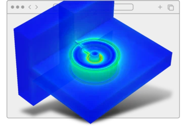
Step 6: Post-Process and Extract Results
In the post-processor, visualize the transient flux density magnitude across the flyer tube and inner rod. Extract additional outputs: ohmic losses, electric current density, and field data. Time-transient force data can be downloaded for further analytical calculations (e.g., computing impact velocity of the flyer).
Results: Conductivity Sweep (30%–60% IACS)
Force: Maximum total Lorentz force on the flyer increases slightly with conductivity, but the change is modest. Magnetic pressure is relatively stable across the tested range.
Current density: Increases significantly with conductivity as the skin depth decreases, concentrating the current in a thinner surface layer. While higher conductivity leads to stronger eddy currents and higher peak current densities (J), it simultaneously reduces electrical resistance (R), typically resulting in lower overall Ohmic losses . In MPW, the primary thermal risk is not electrical heating, but rather the adiabatic heating generated by high-velocity plastic deformation and impact at the weld interface.
Shielding: Flux density on the flyer’s outer surface is significantly higher than on the inner surface due to the opposing magnetic field generated by the eddy currents (electromagnetic shielding). This effect becomes more pronounced at higher conductivities.
Takeaway: While forces are stable, switching Al grades significantly alters the Impact Dynamics. Higher conductivity leads to higher velocities for a given voltage. Rather than thermal monitoring, focus on calibrating discharge energy to account for the varying plastic work and adiabatic heating of different alloys.
Results: Air Gap Sweep (0.9 mm vs. 0.4 mm)
| Parameter | 0.9 mm gap | 0.4 mm gap |
|---|---|---|
| Total Lorentz force on flyer | ~8 kN | ~9 kN |
| Peak flux density in gap | ~25 T | ~28–29 T |
Reducing the air gap from 0.9mm to 0.4mm significantly tightens the electromagnetic coupling, resulting in a 16% increase in peak flux density and a 12.5% increase in Lorentz force.
Therefore, a few millimeters of tooling misalignment shifts force output and flux density enough to affect weld quality. Use these sensitivity curves to define acceptable tolerance bands for production tooling. With a smaller air gap, the outcomes may differ further — worth investigating depending on your field shaper geometry.
Thermal Coupling
Extend the simulation with thermal coupling to map electromagnetic ohmic losses as heat sources in a thermal analysis. This verifies the flyer tube and inner rod don’t approach melting during the process.
| Parameter | Value |
|---|---|
| Peak flyer tube temperature | ~450 °C |
| Al melting point | ~660 °C |
| Margin | 210 °C |
The process stays within safe thermal limits. The time-transient force data can be downloaded and used for analytical calculations to determine the impact velocity and verify sufficient kinetic energy for the weld.
Support and Collaboration
SimScale provides support at every stage of the simulation workflow. The platform includes an AI assistant trained on SimScale documentation, tutorials, and case studies, as well as direct access to support engineers for tailored advice on your specific simulation setup.
For team workflows, share any project with colleagues regardless of their location — no data download/upload required. Grant view, copy, or edit access directly from the platform.