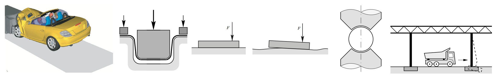
All movements that occur on this planet involve contact mechanics and friction. Consider even the simplest acts like walking, driving a car, riding a bicycle, all the way up to powerful steam trains. Such physical problems involving contact mechanics are not only common in mechanical and civil engineering industries, as shown in Figure 1, but also in environmental and medical applications like cardiovascular stents, hip replacements, pollution due to wear particles and more.
Studies of Contact Mechanics and Friction through Ages
The importance of friction and contact mechanics was identified long ago. As shown in Figure 2, hieroglyphics show that ancient Egyptians knew about lubrication because when they moved large stones, liquid was frequently poured in front of the sledge to reduce friction. The ancient Indian civilization used hard stones like granite in the construction of buildings like the Brihadeshwar temple. Granite is one of the hardest stones to cut and they knew that contact stresses could be exploited for cutting. Dry wooden wedges were inserted into adjacent holes, drilled from blunt chisels, and further watered. When the wedges expanded, the contact stresses cracked the granite.

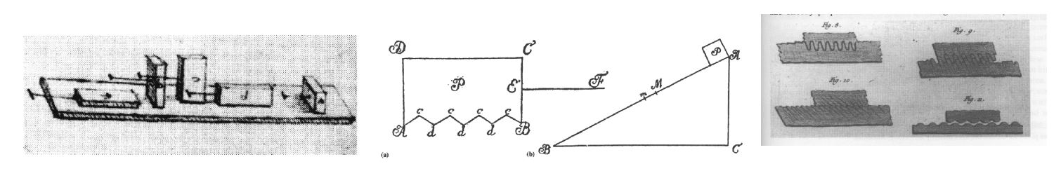
Contact mechanics and friction have been studied since the 15th century by great scientists like da Vinci, Coulomb, and Euler. Figure 3 shows some of their devices or ideas related to contact and friction.
Due to the nonlinear nature of contact mechanics, such problems are often approximated by special assumptions or boundary conditions. Contact mechanics and friction have been studied for several centuries and are still the toughest unsolved problems of solid mechanics. Due to the rapid growth of computational power, today we can use the ideas of computational mechanics to numerically simulate applications of contact mechanisms for sufficient design accuracy. Yet, even to this day, none of the standard finite element software is fully capable of solving contact problems, including friction, with robust algorithms. Hence, computational contact mechanics continues to remain a challenge for the finite element community.
Contact Mechanics on the SimScale Platform
SimScale provides robust methods for enforcing contact constraints during FEM simulation. The numerics related to contact are brought through Code_Aster and CalculiX. Contact constraints are enforced through two mathematical techniques called the penalty method and augmented Lagrangian method.
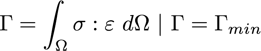
When a displacement or force is applied to a body during a finite element simulation, the body can be deformed into several possible configurations. However, it always results in the same unique configuration! The reason being that the deformation is governed by the principle of energy minimization. When a force or displacement is applied, external work is done on the body. By conservation of energy, this energy is stored in the body as strain energy (stress x strain). Now, the strain (or deformation) is such that the total strain energy is as minimal as possible. For a simple linear elastic case, this can be written as:
Now, when two surfaces of the body (or multiple bodies) are in contact, then the surfaces are under compressive loading. If the loading is later increased, there can be a nonphysical interpenetration, which should be avoided. Hence, when there is such a nonphysical interpenetration, some extra energy is added. Since the goal is to look for a minimum energy, the system will try to avoid the addition of such energy contributions due to interpenetration. As a result, a constraint is imposed on the system that the two surfaces can be in contact but cannot penetrate each other. With this additional energy contribution, and owing to this contact (or when interpenetration happens), the total energy can be written as:

There are many approaches to writing this energy contribution from contact. In SimScale, Penalty and Augmented Lagrange approaches are available. Before discussing these approaches, it is imperative to understand some standard terms like gap function and pressure that are frequently used in this context.
Kinematics of Contact
Work or energy can be defined as force times displacement. During contact, the pressure (normal force) on the surface in contact is p and tangential force, in the presence of friction, is tT. The distance between the two surfaces along the normal direction is gN and along the tangential direction is gT as shown in Fig. 04.
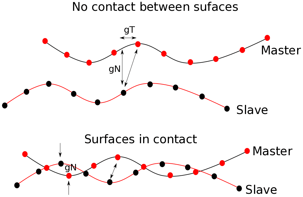
So, for a simple normal contact, the work done can be written as p x gN. If there is no friction, there are no tangential stresses and hence no contribution from that. In the presence of friction, additional work contribution due to friction is added as tT x gT.
The above is concisely written in terms of the Signorini-Hertz-Moreau condition:
- When there is no contact, forces are zero, but the gap is positive. Thus, no work is added.
- When there is contact, forces are non-zero, but the gap is zero. Thus, no work is added.
- When there is interpenetration, the gap is negative and the pressure is non-zero. Thus, additional energy is added such that gap returns to zero in the subsequent iterations.
Penalty Method
When the penalty method is employed, as shown in Figure 5, an ad-hoc penalty coefficient is assigned by the user.
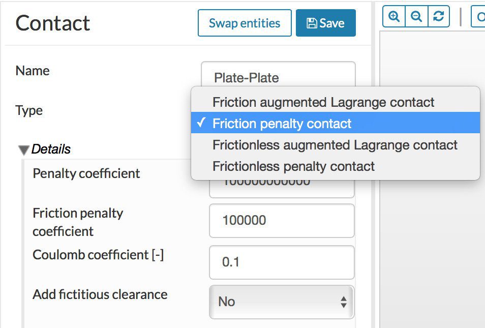
The recommended value for the penalty coefficient is generally about 1-100 times the Young’s modulus of the material. Similarly, the friction penalty coefficient is assigned to the tangential direction. The penalty parameter is a scaling factor to calculate the normal pressure, but only when there is contact or interpenetration, as:
Normal pressure = Penalty coefficient x gN
Tangential force—or actually tangential traction—can similarly be calculated for sliding using the friction penalty coefficient. If there is an interpenetration, gN < 0, which results in a compressive pressure. Now, the change in energy contribution as a result of contact due to a small change the gap can be given as:

and this is always greater than or equal to zero. Thus, the only possible minimum point is when the gap (gN) is zero. As the penalty parameter increases to infinity, the energy also increases and the contact is imposed exactly. However, large penalty parameters lead to “ill-conditioning”, which makes it harder to reach convergence. For this reason, the recommended value for the penalty parameter is about 10-100 times the Young’s modulus of the material.
Augmented Lagrangian Method
In order to circumvent the problem of ill-conditioning, the Lagrange multiplier method was explored. In this instance, the pressure (or the tractions) are considered as unknowns and are iteratively solved as additional unknowns. Now the change in energy contribution as a result of contact due to a small change in the gap can be given as:

Here the pressure p is also considered unknown and solved for. Correspondingly, the total size of the problem increases, which can add substantial costs depending on the number of elements that are in contact.
Contact is a nonlinear problem. This means that it is not known a priori if an interpenetration exists at a point. During the iteration, each point is checked for interpenetration and, in such a case, an extra constraint is added. This means that a point that was not undergoing interpenetration at an earlier iteration could now be interpenetrating in this iteration. So each point on a possible contact surface iterates between in-contact and no-contact. In this transition zone, the Lagrange multiplier can demonstrate an oscillatory behavior.
The augmented Lagrangian method was formulated to provide the benefits of both the penalty and the Lagrange multiplier. However, it does not demonstrate an oscillatory behavior and has minimal interpenetration. The change in energy contribution for a small change in the gap can be given as:

where the variables are the same, just as described earlier.
Here, the penalty parameter is called “augmentation coefficient”. The Lagrange multiplier “p” is an unknown and calculated during the solution process. The above has been explained for a normal contact. Similar arguments can be constructed for tangential contact involving friction. For a more detailed mathematical discussion of these topics, the reader is referred to References [2] and [3].
Discover all the simulation features provided by SimScale. Download the document below.

Numerics: Choosing the Best Option
Finally, getting to the hands-on part. SimScale offers exciting options to simulate contact in structural mechanics simulations as shown in Figure 7.
Tip 01: Mesh Refinement
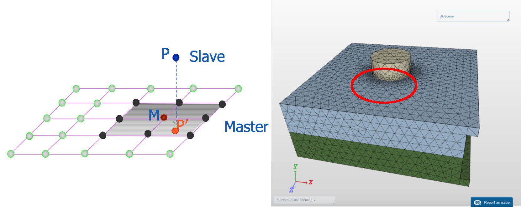
At present, SimScale uses a node-to-surface formulation, as shown in Figure 8. A perpendicular is dropped from each node on the slave surface to the master surface. This is used to put necessary distance between the slave node and the master surface. This formulation, at present, is stable for small sliding only. Thus, the mesh at the contact surfaces needs to be well refined, as demonstrated in the bolt connection example in Fig. 08.
Tip 02: Penalty or Augmented Lagrangian Method?
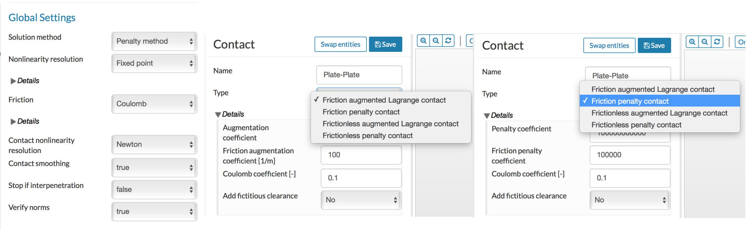
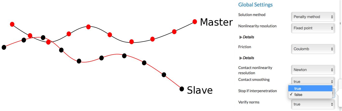
The global option is the selection of penalty or augmented Lagrangian method, as shown in Figure 9.
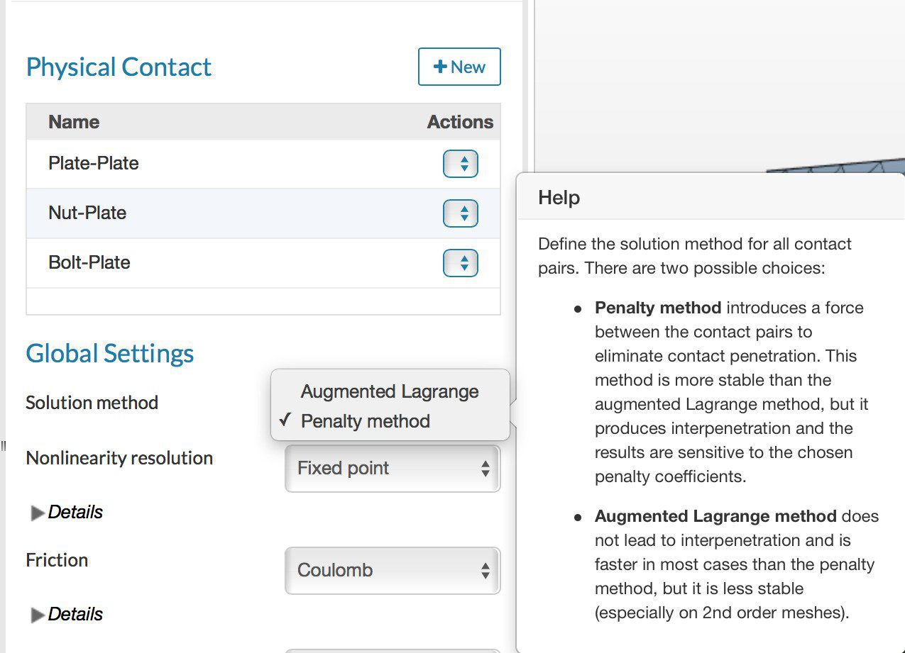
As indicated in the above tip, the penalty method produces a small interpenetration, while the augmented Lagrange method is almost exact. That apart, the penalty method is generally sufficient for most problems that involve small sliding. The augmented Lagrangian method could be used for improved accuracy in problems with less than 100,000 nodes. For larger problems, however, it would be necessary to note the number of elements/nodes in the contact region, since this contributes to an increase in the total equation size.
Tip 03: Friction
Friction can be an important factor in several physical applications and cannot be neglected. There are some applications where friction can be neglected, and the results are still acceptable for preliminary design purposes.
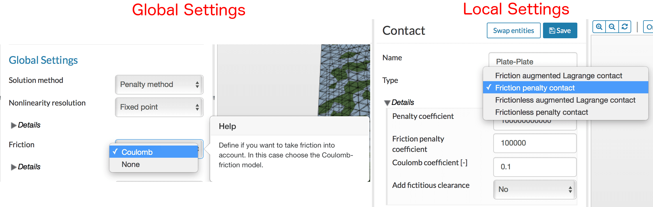
SimScale presently offers consideration of friction through the Coulomb friction law, as shown in Figure 10. Correspondingly, if friction is chosen, the frictional penalty or frictional augmented method needs to be selected in the local contact settings. If the global settings do not use friction, then frictionless options should be selected in the local settings.
Tip 04: Contact Smoothing
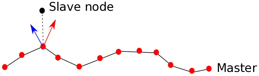
As shown, the slave node, when projected, could be associated with the two different master surfaces. This situation could be common and lead to convergence issues when first-order elements are being used. Using the contact smoothing option allows for smoothing of the associated normals and prevents such ambiguities.
Tip 05: Stop if Interpenetration
SimScale offers one-of-a-kind options that are generally not found in many commercial and academic codes. One of the very common reasons for the failure of contact simulations is the presence of interpenetration. When there is an interpenetration, and it isn’t resolved after several iterations, the residual continues to remain beyond the threshold and the simulation crashes.
In most scenarios, the interpenetration is only at a few nodes (as in Figure 12), and they would likely resolve in the next subsequent time step(s). In such a situation, it is likely that this option could be very helpful.
However, this option needs to be used with extreme caution. As often said, “with great power comes great responsibility!”. When this option is used, one must make a critical assessment of the accuracy of the results.
Tip 06: Verify Norms
Just like the contact smoothing option, verifying the surface norms can be extremely helpful, as it ensures that the normals are continuous. This is particularly preferred when first-order meshes are used.
Constraint between Contact Surfaces
In addition to the above, there are situations when the contact surfaces do not undergo relative motion. For example, two surfaces could be glued, symmetry could exist, or only sliding—but not normal—displacement could be allowed between the surfaces.
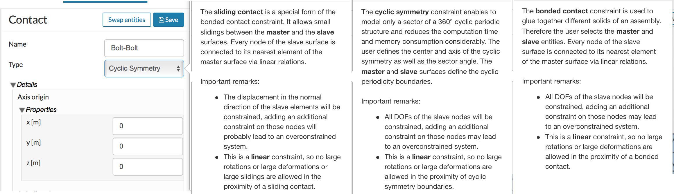
Cyclic symmetry exploits symmetry, while bonded symmetry can be used when two surfaces, made of different solids in the assembly, are glued. In contrast, sliding contact can be used when there is no normal opening, but sliding is allowed between the surfaces. These conditions can be used only when the sliding is small.
Concluding Remarks
Computational contact mechanics remains one of the biggest challenges related to solid mechanics. The problem formulation is strongly nonlinear and beyond what is observed in most structural problems. SimScale offers several options that allow robust algorithms for structural simulations that involve contact. Long gone are the days when contact had to be approximated by special assumptions or boundary conditions.
References
- SimScale documentation: Physical contacts, Contact constraints
- Peter Wriggers, Computational Contact Mechanics, Springer-Verlag Berlin Heidelberg
- Alexander Konyokhov and Ridvan Izi, Introduction to Computational Contact Mechanics: A Geometrical Approach, John Wiley and Sons
Download this case study for free to learn how the SimScale platform was used to investigate a ducting system and optimize its performance.