Turbulence: Which Model Should I Select for My CFD Analysis?
written by
Serkan Solmaz
updated on
April 1st, 2026
approx reading time
7 Minutes
BlogCFDTurbulence: Which Model Should I Select for My CFD Analysis?
“Turbulence is the most important unsolved problem of classical physics.” (Richard Feynman, American theoretical physicist, Nobel Prize in Physics in 1965)
“I am an old man now, and when I die and go to heaven, there are two matters on which I hope for enlightenment. One is quantum electrodynamics, and the other is the turbulent motion of fluids. And about the former, I am rather optimistic.” (Horace Lamb, English applied mathematician, Advisor: George Gabriel Stokes)
Even a few decades after these great scientists expressed these remarks, turbulence modeling is still no easy thing. If you’re just getting started, our introduction to CFD analysis covers the fundamentals before diving into turbulence model selection.
Set up your own cloud-native simulation via the web in minutes by creating an account on the SimScale platform. No installation, special hardware, or credit card is required.
The idea of using fluid to extract or deliver energy is not recent. In the 17th century, Leonardo Da Vinci conducted various experiments to visualize fluid flow, talking about vortex flow, vorticity, swirls, and eddies.
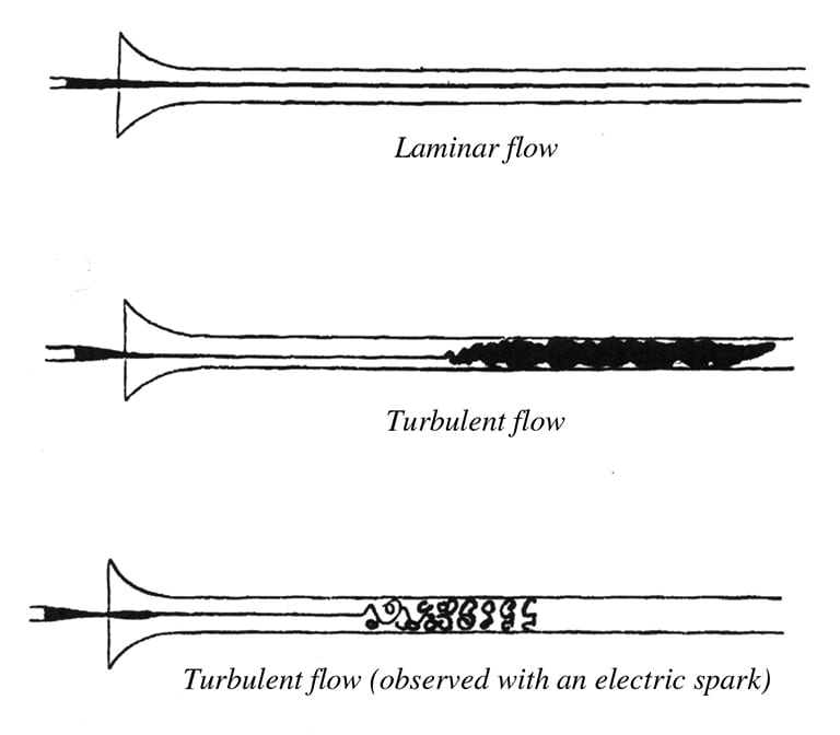
Figure 1: Experimental visualization conducted by Osborne Reynolds [1] (Source: By Osborne Reynolds (Scan from book) [Public domain], via Wikimedia Commons)
Fluid flow is classified into two main categories—laminar or turbulence—regarding the driven forces (inertial, viscous, etc.), and also a transition regime between them. Notably, being laminar or turbulent is a property of fluid flow under dynamic conditions, not a property of being fluid.
Laminar Flow: A fluid flows through a smooth path with no disruption between adjacent paths. It is quite compatible to examine laminar flow both numerically and experimentally.
Turbulent Flow: A fluid flows through a chaotic path that comprises eddies, swirls, and flow instabilities. It is uneasy, almost impossible in some cases, to examine turbulent flow both numerically and experimentally.
Earlier, the determination of the type of fluid flow numerically was hard to realize. Irish scientist Osborne Reynolds (1883) discovered the dimensionless number that predicts fluid flow based on static and dynamic properties such as velocity, density, dynamic viscosity, and length:
Re=(inertial force)/(viscous force)=ρVL/μ
Where ρ (kg/m3) is the density of the fluid, V (m/s2) is the characteristic velocity of the flow, L (m) is the characteristic length scale of flow, and μ (Pa*s) is the dynamic viscosity of the fluid.
Type
Flow type
Reynolds Number
Internal
Laminar regime
up to Re=2300
Transition regime
2300<Re<4000
Turbulent regime
Re>4000
External
Laminar to Turbulence
Re>3×10⁵
Table 1: Flow types according to the Reynolds number
If the inertial forces—which resist a change in velocity of an object and cause of the fluid movement—are dominant, the flow is turbulent. On the contrary, if the viscous forces, defined as the resistance to flow, are dominant, the flow is laminar. It is common to generate turbulence for a fluid with low viscosity, though it is rare for fluids with high viscosity. A detailed description of the Reynolds number can be obtained from the SimWiki: What is the Reynolds number?
Aside from laminar behavior, turbulence encompasses several hurdles, and thus requires rigorous effort during experimental and numerical examinations. Turbulence is a type of fluid flow which is unsteady, enormously irregular in space and time, three-dimensional, rotational, dissipative (in terms of energy), and diffusive (transport phenomenon) at high Reynolds numbers. Due to those divergences in turbulent flow, extremely small-scale fluctuations emerge in velocity, pressure, and temperature. Despite the fact that direct implementation of fluctuated values into the Navier-Stokes equation is possible, called a Direct Numerical Solution (DNS), it requires an extreme amount of resources in terms of hardware, software, and human effort. Therefore, an appropriate numerical model should be implemented when modeling turbulent flow.
Figure 2: The velocity fluctuation in turbulent flow [2]
In this case study, the SimScale cloud-based CAE platform was used to investigate a ducting system and optimize its performance. Download it for free to learn how.
Which turbulence model is convenient for your CFD analysis is a troublesome question. To select an appropriate model and simulate physical incident as accurately as possible, you must:
Scrutinize the physical incident to understand the phenomenon
Research the literature in detail to define a suitable model
If literature is poor, try some models concurrently to get an accurate prediction
In the validation process, take care of the model that you would apply
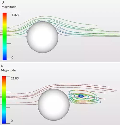
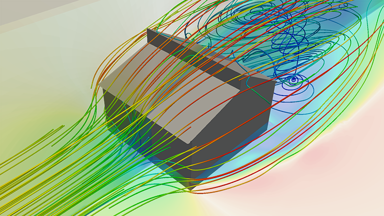
Figure 3: Laminar (up) and turbulent (down) flow – CFD analysis results for a geometry
Implementation of the turbulence model into the numerical scheme is substantial and makes a big difference to the simulation results. At the first step, a quick examination must be carried out—which pertains to the Reynolds number—to detect the type of fluid flow. For instance, as you keep on with the laminar model (no turbulence) for a fluid flow over a cylinder which is turbulent in the reality, the effect of the driven forces, eddies, vorticities and so forth are destructively negated. The numerical study hereby diverges, as demonstrated in Figure 3.
Although there is a number of miscellaneous turbulence models that investigate the motion of the fluid, these rely on turbulent viscosity, and no universal turbulence model exists yet. Generally, turbulence models are classified regarding governing equation and numerical method used to calculate turbulent viscosity, for which a solution is sought for turbulence. Reynolds-averaged Navier-Stokes equations (RANS) and large eddy simulation equations (LES) are the common ones that require a compatible amount of resources during examination against DNS. Beyond that, Unsteady Reynolds-averaged Navier-Stokes (URANS), in which motion of the solid body or flow separation causes unsteady flow, has been broadly implemented.
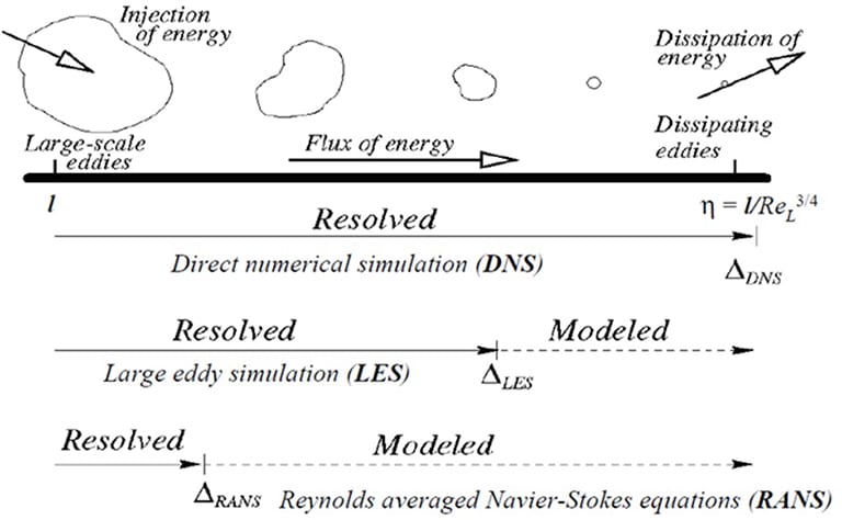
Figure 4: Ability of methods to solve according to the scale of eddies within a model
The main purpose of turbulence modeling is to prompt equations to anticipate the time-averaged velocity, pressure, and temperature fields, without calculating the complete turbulent flow pattern as a function of time as in RANS and LES. It is unnecessary to solve the Navier-Stokes equations for every value of fluctuation since most engineering problems do not require such a comprehensive solution. The turbulence models can be summarized as follows:
DNS: Direct implementation of fluctuated values into the Navier-Stokes equation without any turbulence model.
LES: An average turbulence model between DNS and RANS in which filtered Navier-Stokes equations are used for large-scale eddies. An appropriate model is preferred to solve small-scale eddies.
RANS: A mathematical model based on average values of variables for both steady-state and dynamic flows (unsteady for URANS). The numerical simulation is driven by a turbulence model which is arbitrarily selected to find out the effect of turbulence fluctuation on the mean fluid flow.
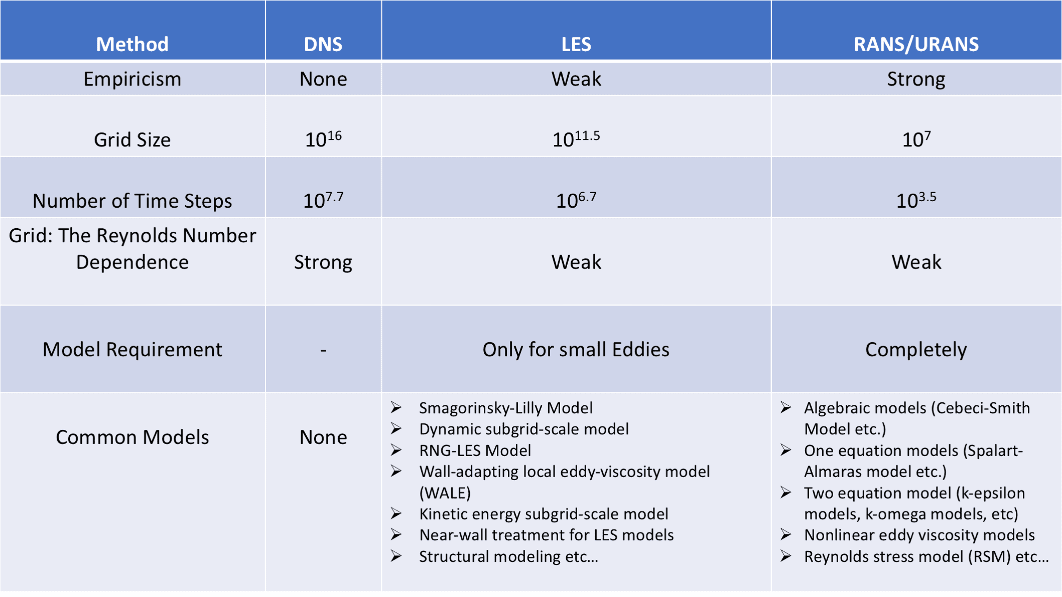
Table 2: Comparison of turbulence models/methods
Commonly Applied Turbulence Models in CFD Analysis
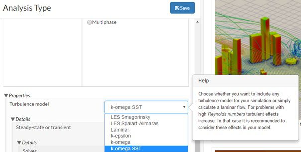
Figure 5: The SimScale environment – turbulence models for CFD analysis
Requiring a modest amount of hardware, computational time, and human effort, RANS/URANS methods, and sub-models are highly applied for various computational fluid dynamics problems. The implementation of LES is rare but possible in some cases which specifically need much more computational facilities against URANS/RANS. Here are the most prominent turbulence models you can run in the SimScale environment:
Spalart-Allmaras
One-equation model
No wall functions
Stable with good convergence
Convenient: Aerodynamics flows, transonic flows over airfoils
CFD analysis of turbulent flow over a house carried out with SimScale
I hope this article helped you better understand turbulence. If you’d like put your knowledge into practice and set up your own CFD analysis, SimScale offers the possibility to carry out simulations in the web browser. To discover all the features provided by the SimScale cloud-based simulation platform, download this document. In addition, here are a few resources that you might find interesting:
Reynolds, Osborne. “An experimental investigation of the circumstances which determine whether the motion of water shall be direct or sinuous, and of the law of resistance in parallel channels”. Philosophical Transactions of the Royal Society. 174 (0), 1883, P. 935–982
Bird, R.B., Stewart, W.E. and Lightfoot, E.N. “Transport Phenomena”, 2ndth edition, John Wiley & Sons, 2001, ISBN 0-471-41077-2
Stay updated and never miss an article!
Other 'CFD' Stories
Your hub for everything you need to know about simulation and the world of CAE
![Figure 2: Turbulent flow and fluctuation in velocity [2].](https://frontend-assets.simscale.com/media/2017/07/figure2-e1499332975945.jpg)