Boundary Conditions
Boundary conditions define how a system, ( for example, a structure or a fluid ), interacts with the environment. Fixations, loads, pressures, flow rates, or velocities are all examples of boundary conditions.
A boundary condition consists of three pieces of information:
- Boundary condition types: SimScale offers a large set of boundary condition types for simulations. This section links to descriptions of the available boundary condition types.
- Boundary condition assignments: A boundary condition is usually only assigned to the domain’s boundary. Each boundary condition must be linked to at least one surface or where something enters or exits the domain.
- Boundary condition values: This is where we define the value of the condition (speed, temperature, force, etc.);
Boundary Condition Types
SimScale offers many boundary condition types for different types of applications. Boundary conditions are only displayed when they can be applied to the type of analysis being worked on. The following list shows the available boundary condition types, what each type means, and where they can be used. For advanced users, the page also shows how the boundary condition types translate to the solver input files.
Fluid Dynamics
- Custom
- Empty 2D
- Fan
- Natural convection inlet-outlet
- Periodic
- Pressure inlet and Pressure outlet
- Symmetry
- Velocity inlet and Velocity outlet
- Wall
- Wedge
- Atmospheric boundary layer inlet
Solid Mechanics
- Base excitation
- Bolt preload
- Centrifugal force
- Cyclic symmetry
- Hinge constraint
- Elastic support
- Fixed support
- Fixed value
- Follower pressure
- Force
- Nodal load
- Point mass
- Distributed mass
- Pressure
- Remote displacement
- Remote force
- Rotating motion
- Surface load
- Symmetry plane
- Volume load
Thermodynamics
Electromagnetics
- Fixed potential
- Floating potential
- Charge density
- Total charge
- Magnetic field normal
- Magnetic flux tangential
- Radiation heat flux
Creating and Assigning a Boundary Condition
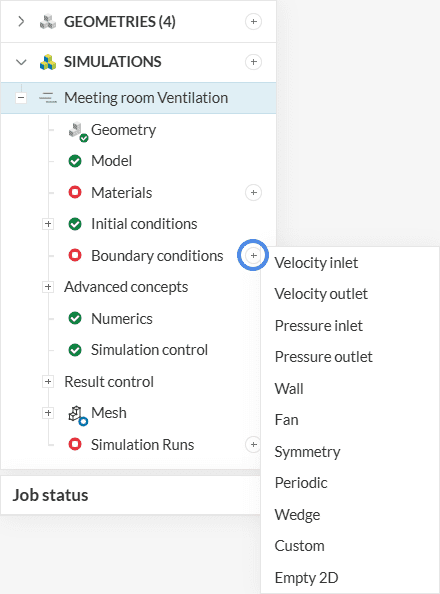
To create a new boundary condition, click on the ‘+ button‘ next to Boundary conditions. Pick the desired one from the list:
After creating a boundary condition, assign the desired entities by clicking on them.
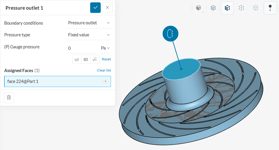
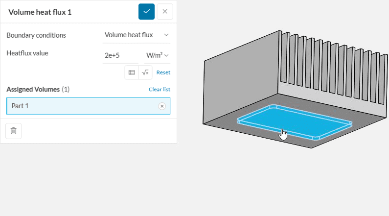
All of the fluid dynamics boundary conditions are assigned to faces exclusively. For solid mechanics and thermodynamics, some boundary conditions can only be assigned to volumes, such as Volume heat flux.
Lastly, some of the solid mechanics boundary conditions accept assignments of both faces and volumes, such as the Rotating motion boundary condition.
Boundary Condition Values
For simple cases, boundary conditions are defined by a single value of a given variable (velocity, temperature, pressure…). For advanced cases where a fixed value is not enough, alternative techniques are available:
Boundary Condition Visualization
The boundary condition visualization tool shows the simulation setup in a visual format, helping users better understand and explain their configurations, especially when creating reports.
Last updated: February 12th, 2026
Did this article solve your issue?
How can we do better?
We appreciate and value your feedback.


