Documentation
This validation case belongs to fluid dynamics. The aim of this test case is to validate the following parameters for a drone propeller:
The simulation results of SimScale were compared to UIUC wind tunnel measurements presented in [1].
The geometry used for this case can be seen below:
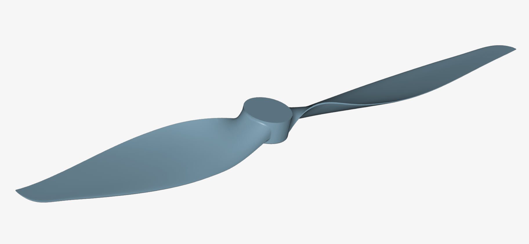
It is a two-blade propeller represented using its dimensions in inches. This APC 11×5.5E model is an 11-inch diameter propeller with a pitch of 5.5 inches/revolution used on small UAVs and model aircrafts.
Tool Type: OpenFOAM®
Analysis Type: Steady-state, incompressible analysis with MRF rotating zone, using the k-omega SST turbulence model.
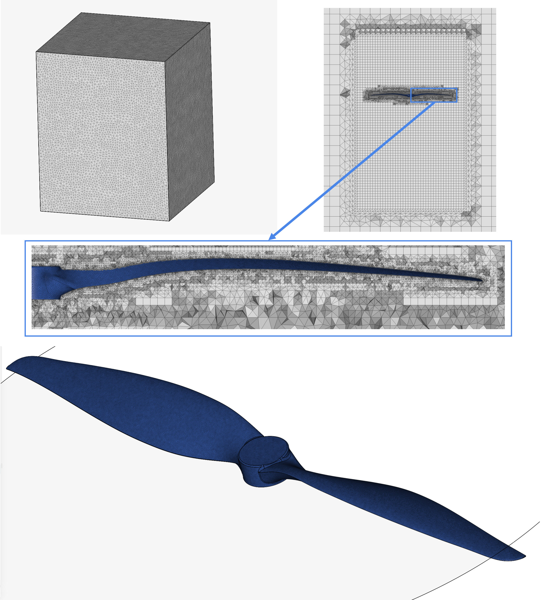
Mesh and Element Types:
The Standard mesher algorithm with tetrahedral and hexahedral cells was used to generate the mesh. Multiple meshes with incrementally increasing refinement were generated in parallel using the automatic meshing functionality.
For each run, the thrust and power coefficients were calculated and plotted below:
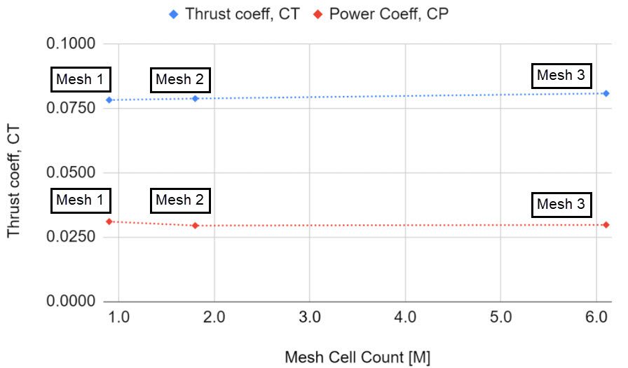
A mesh sensitivity analysis has been carried out monitoring the y+ maximum values while using full resolution wall treatment with the standard mesher:
| Mesh Name | Element Type | Number of cells/nodes | Max y+ |
| Mesh 1 | 3D Tetrahedral/Hexahedral | 4.3M cells, 1.4M nodes | 3.2 |
| Mesh 2 | 3D Tetrahedral/Hexahedral | 6.1M cells, 2.2M nodes | 1.5 |
| Mesh 3 | 3D Tetrahedral/Hexahedral | 13.4M cells, 4.1M nodes | 0.46 |
Material:
Boundary Conditions:
The UIUC\(^1\) data uses the standard definitions for propeller aerodynamic coefficients:
Thrust coefficient:
$$C_T = \frac{T}{\rho \times\ n^2 \times\ D^4}$$
Power coefficient:
$$C_P = \frac{P}{\rho \times\ n^3 \times\ D^4}$$
Where:
Comparison of the thrust and power coefficients obtained from SimScale against the experimental results obtained from [1] is given below:
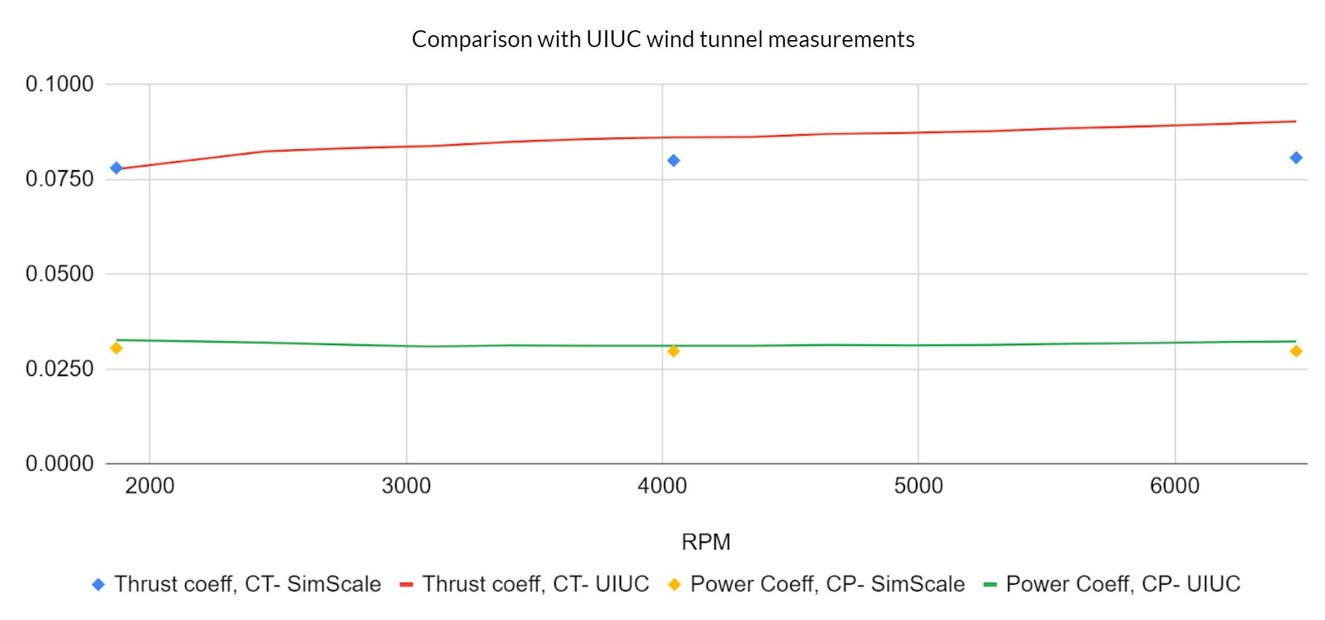
The SimScale results appear to be on track with the wind tunnel measurements, and below the discrepancies are calculated for each run:
| RPM | Thrust Coefficient Discrepancy [%] | Power Coefficient Discrepancy [%] |
|---|---|---|
| 1868 | 0.4272 | 6.5879 |
| 4043 | 7.0814 | 4.6446 |
| 6473 | 10.6043 | 7.8704 |
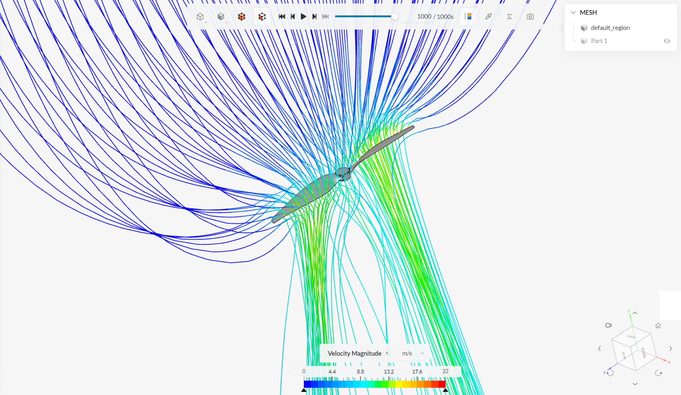
In the following images, the results were analyzed in the post-processor. The streamlines tend to concentrate below the propeller, after being drawn by the propeller’s rotation:
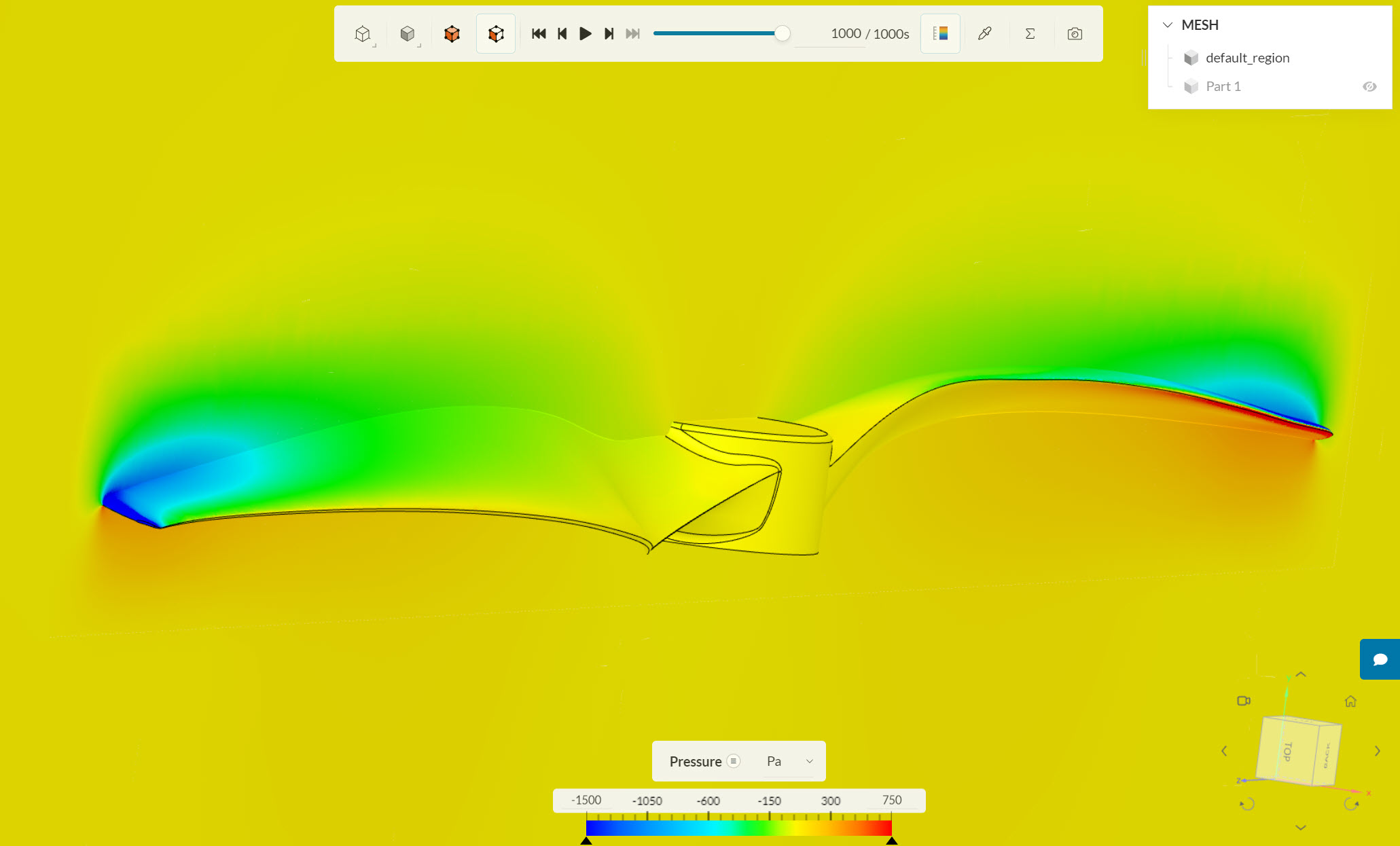
With rotational axis in the negative y-direction, the difference in pressure on the blade is created as shown below:
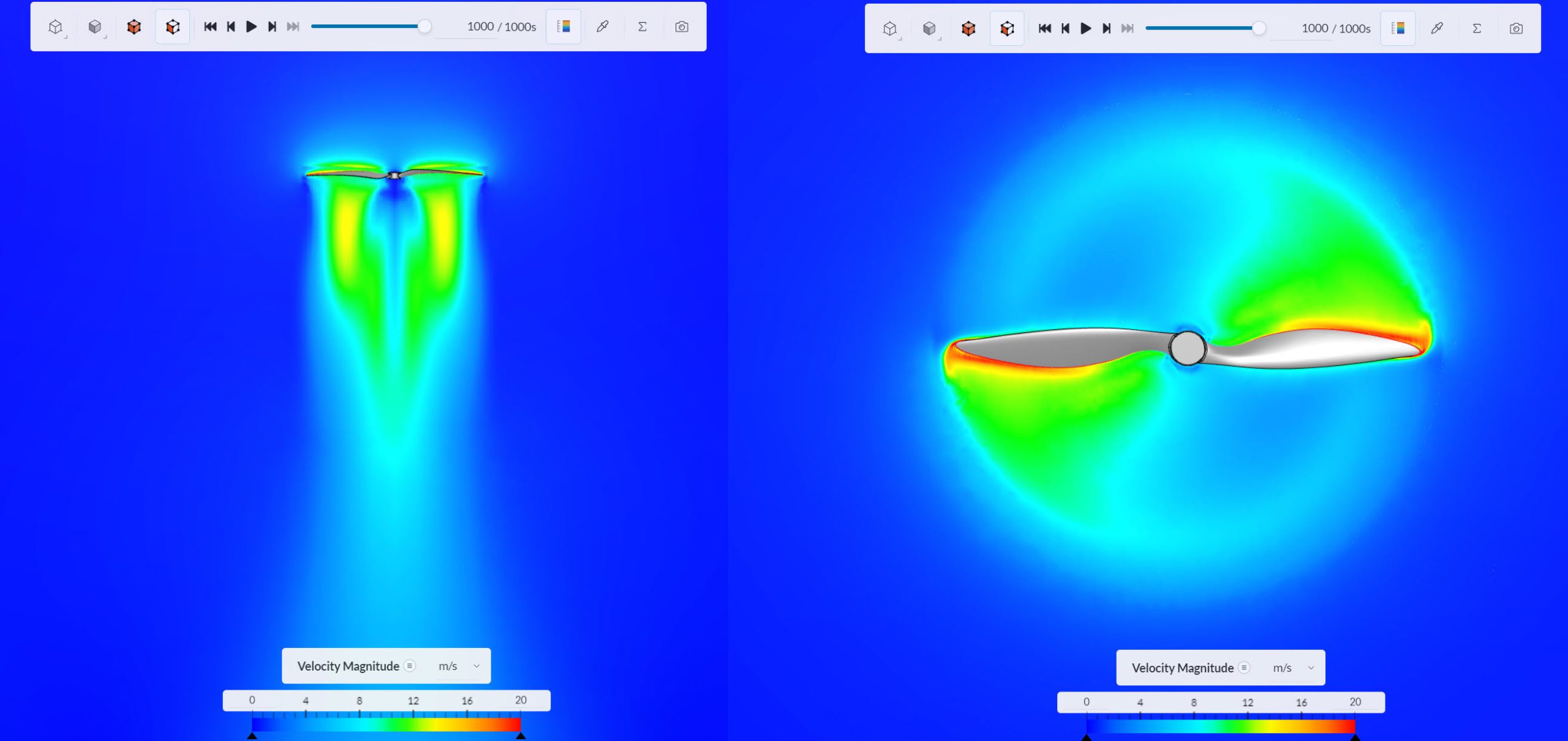
Finally, the following cutting planes showcase the high velocity streams that are formed longitudinal to the flow.
References
Note
If you still encounter problems validating you simulation, then please post the issue on our forum or contact us.
Last updated: April 5th, 2024
We appreciate and value your feedback.
Sign up for SimScale
and start simulating now