Documentation
A simulation was set up and run using the LBM method provided by Numeric Systems GmbH replicating the setup described by the Architectural Institute of Japan (AIJ) for their validation case E. The results showed good correlation to the wind tunnel data provided, where correlation coefficients of between 0.7 and 0.86 were obtained. Solve times were drastically reduced over traditional CFD methods, surprising when we solved them in transient using a k-omega SST DDES turbulent model.
With the increase in the number of high-rise buildings being constructed all around the World, proper planning of the close vicinity for comfort and safety becomes important. Computational Fluid Dynamics (CFD) is an apt solution for assessing these comfort and safety levels for Pedestrian Wind Comfort even before the buildings are erected and also helps in faster design iterations. Pedestrian-level (micro-climate) condition is one of the first microclimatic issues to be considered in modern city planning and building design\(^1\).
Wind analysis results using CFD simulation are now seen as reliable sources of quantitative and qualitative data, and they are frequently used to make important design decisions. However, to have full confidence in those decisions, extensive verification and validation of the CFD results are necessary. For this, we will be validated against the experimental results of some very well documented cases provided by the Architectural Institute of Japan (AIJ).
The Architectural Institute of Japan (AIJ) is a Japanese professional organization for architects, building designers, and engineers. It was founded in 1886 and has gathered over 38,000 members since. It publishes several journals, technical standards for architectural design and construction, and research committee studies.
The wind analysis test case for this validation was taken from the “Guidebook for Practical Applications of CFD to Pedestrian Wind Environment around Buildings”\(^3\), published by AIJ in 2008, which sets the standards for cross-comparison between the results of CFD predictions, wind tunnel tests, and field measurements, and helps validate the accuracy of CFD codes for pedestrian wind comfort assessments.
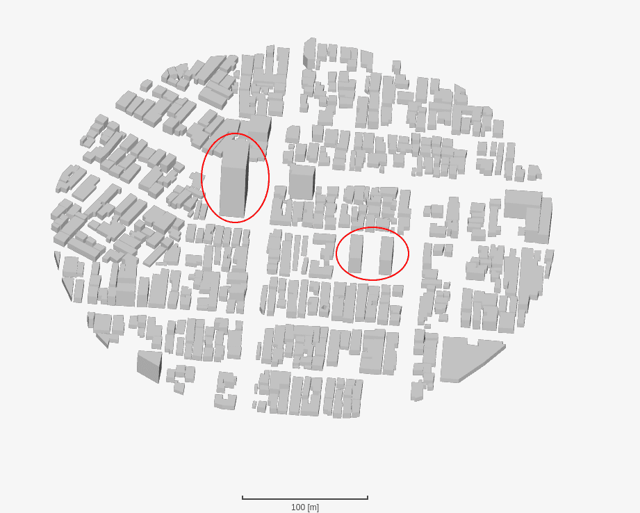
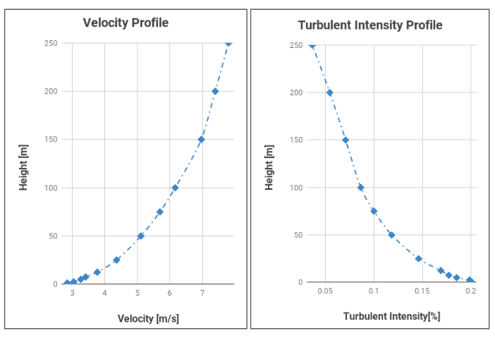
The case being validated is Case E, which is a simplified geometry of a complex of buildings. The urban area model treated here was an actual city block in Niigata city, Japan, with low-rise houses jammed closely together and one target high-rise building at 60m high. Wind tunnel experiments at 1/250 scale were performed on this model in a turbulent boundary layer with a power-law exponent of 0.25.
Out of the many scenarios presented in Case E, the impact of the winds from the north, east, south, and west was used to validate the lattice Boltzmann solver of SimScale.
The below picture shows the AIJ Case E geometry with the main buildings highlighted:
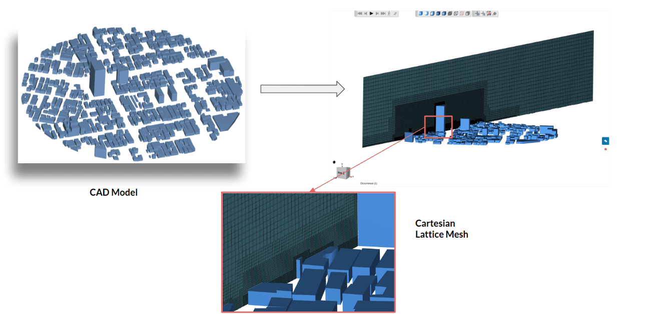
The original CAD model was downloaded as the .DXF file from the AIJ website and converted it to an STL file. This STL file was then imported to SimScale directly and used for simulation.
For this simulation we used SimScale’s LBM solver, which is a different approach to traditional Finite Volume Methods. This solver provided by Numeric Systems GmbH\(^4\) has many advantages over the traditional approach, but the most relevant in this case is geometry robustness, and solve speed. Since the solver runs on GPU architecture, and scales very well, we can solve very large meshes in transient at a fraction of the time it would take traditional solvers to solve in steady state.
A summary of the simulation setup is as follows:
For the simulation, the mesh is optimized with automatic refinements to capture details in the geometry and avoid a large number of cells in unnecessary regions.
As mentioned before we use a turbulence model called K-omega SST DDES which uses the highly regarded LES turbulence model in the far-field but uses the equally well-regarded wall model from the K-omega SST model which has proved its self particularly in the Aerospace Industry. The transition between the two models happens in the log-law region in the boundary layer. This means that we improve turbulence prediction by using LES, but also reduce its inherent cost by adding a robust wall model, reducing the mesh requirement at the wall.
The results shown here are time-averaged over the last 300s of simulated time, they were then normalised by the inlet value at 15.9m and plotted against the results reported by AIJ in the datasheet\(^3\). The plots above show 4 different images. The first (top left) shows where the points in the graphs are located in red dots with their corresponding numbers, the second (top middle) shows the same results with the velocity overlaid at the same height. The third plot (top right) shows how the results correlate, where CFD results from the LBM simulation are plotted on the Y-axis and the experimental results on the X-axis, a perfect plot would be a line with a gradient of 1. Finally, the last plot, considered the main graph is along the bottom, this shows the two sets of data (experimental and CFD) plotted against point number showing exactly how well the results compare, and where it deviates.
The results are plotted for each of the main directions, Northerly, Southerly, Easterly and Westerly wind directions.
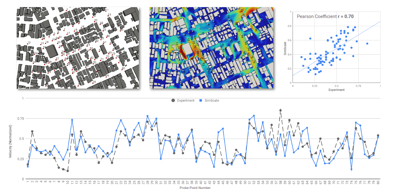
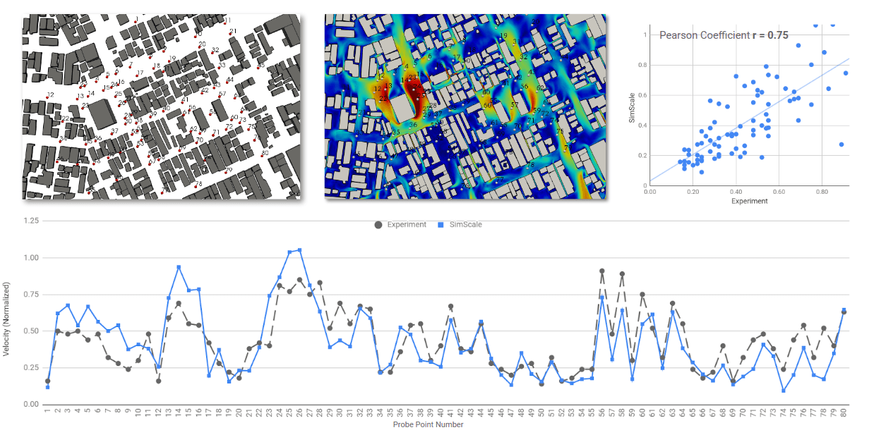
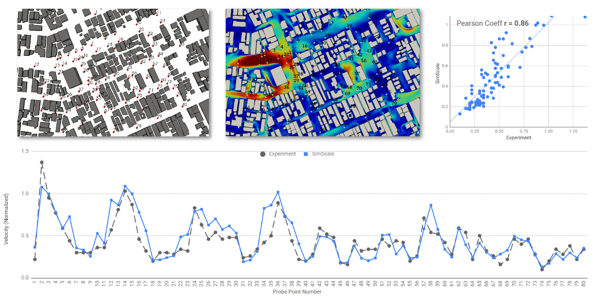
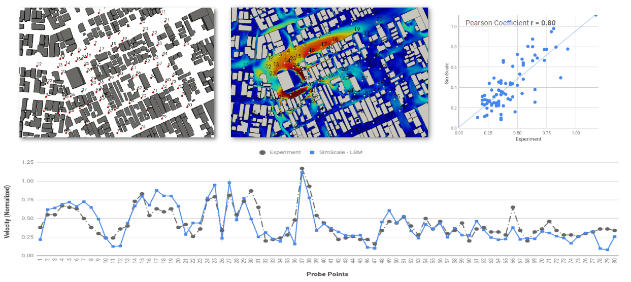
Firstly, lookig at the correlation plots (top right) you can see the ‘Pearson Coefficient r’ shows how the correlation looks for each direction, where they range from 0.7 (Northerly) to 0.86 (Westerly). Furthermore, the correlation can be directly compared looking at the bottom plot, where the results look very similar, and show the correct trends, variation and values.
The advantages of using the Lattice Boltzmann method (Pacefish®) compared to more traditional methods such as our Finite Volume Method powered by OpenFOAM® is that it solves much faster, due to using GPU’s and being more scalable, and accuracy due to using more accurate turbulence models that need to be solved in transient Simulations. The solve times can be reduced by the order days to hours, reducing wait times and cost.
The background, setup and results from running the documented AIJ Case E validation study were presented, where the LBM solver showed good correlation with wind tunnel results provided. The correlation quality was given using the Pearson coefficient where the coefficient ranged from 0.7 to 0.85. All the trends and values of the average results were compared to the corresponding experimental results where we can say that not only is the correlation good, but the trends also look comparable, to the point where we could draw good conclusions on pedestrian comfort.
The speed of the solver in comparison to finite volume methods was evident when the case was solved in 10 hours, in comparison to 2-3 days for a significantly smaller mesh in steady-state in openFOAM®. This will allow a much faster solve, with higher accuracy, in shorter amounts of time, which is what we need when solving many directions at once and sets the expectation for how it will scale in the Pedestrian Wind Comfort Analysis type.
References
Last updated: February 18th, 2026
We appreciate and value your feedback.
Sign up for SimScale
and start simulating now