In FEA harmonic dynamics simulations, the input and output quantities typically follow the “harmonic” behavior that dictates the name; that is, the time history for one variable can be expressed as a cosine function of time.
For the result fields of harmonic simulations, this is true in variables that are linearly proportional to the input loads, such as:
- Displacement components
- Strain components
- Stress components
On the other hand, derived quantities expressed as nonlinear functions of the result fields naturally do not exhibit a harmonic behavior. This applies, for example, to:
- Total displacement
- Principal strains and stresses
- Von Mises stress
- Tresca stress
Moreover, the harmonic quantities are expressed in terms of their peak value (module or magnitude are terms used interchangeably for it) and a phase delay angle. This expression is encoded in a single complex number, often called a “phasor.”
In a practical sense, a harmonic quantity at any point will oscillate between a maximum and a minimum value given directly by the module of the response. Therefore, this value can be directly used in engineering assessments, e.g., to know the maximum deflection, maximum strain, peak bending stress, etc.
In contrast to this direct method, an issue arises when the analyst is required to perform their assessment using one of the nonlinear derived quantities, for example, maximum von Mises stress. In this case, the simple harmonic peak value evaluation is no longer available, and a more involved process is needed in order to provide an equivalent simple measure, a.k.a. the “Maximum over phase.”
Max Over Phase Von Mises Stress in SimScale
A feature to compute the max over phase von Mises stress in FEA harmonic simulation results was recently released in SimScale. This feature leverages the analytic formulation of the von Mises stress as a function of the principal stresses to find its maximum value across one harmonic phase cycle. The method first finds the phase sweep angle at which the peak value occurs and then computes the value. Only the max over phase value is delivered in the result fields.
In this study, this feature is tested qualitatively and quantitatively for the accuracy of the results by essentially comparing them to a brute force phase sweep history expansion. All the details of the approach are provided below.
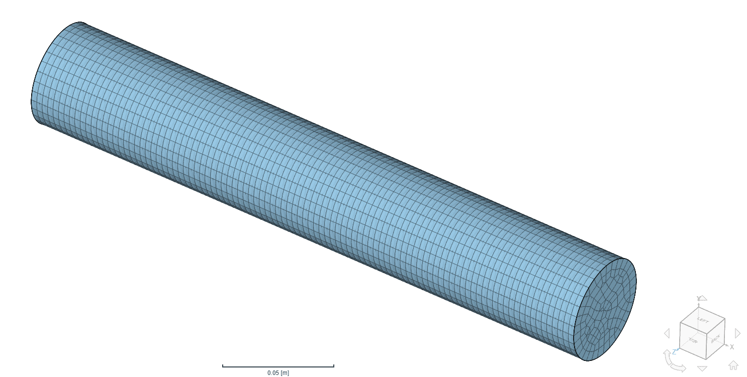
Test Case
The test model captures a round shaft in a cantilever bending configuration. The bending load rotates around the center axis of the shaft while staying orthogonal to it.
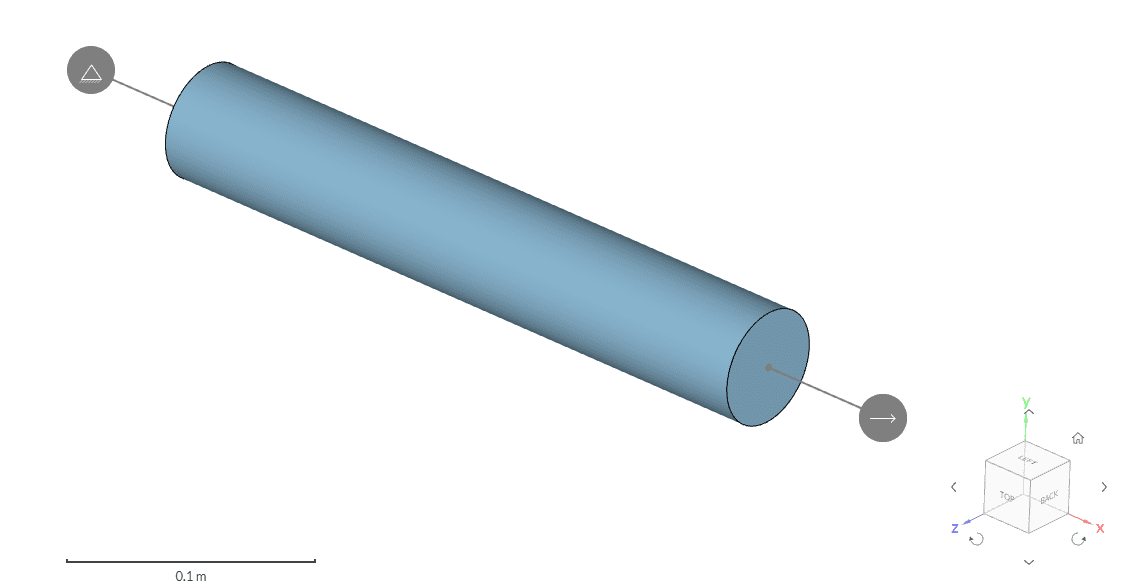
The parameters of the model are:
- Geometry
- Length = 0.3 m
- Diameter = 0.05 m
- Material
- Young’s modulus = 2.05e11 Pa
- Poisson ratio = 0.28
- Density = 7850 kg/m3
- Load
- Peak value = 1000 N
- Direction = orthogonal to the shaft axis
- Vibration = 500 rotations per second
FEA Model
The rotating load is modeled as two orthogonal components spaced at a 90° phase angle:
$$ \vec F = \{F_x, F_y, F_z\} $$
$$ F_x = 0 $$
$$ F_y = 1000 @ 0° $$
$$ F_z = 1000 @ 90° $$
The FEA mesh is implemented with a sweep refinement, giving the following statistics:
- Number of nodes = 49,767
- Number of elements = 11,400
- Tetrahedrals = 0
- Hexahedrons = 10,600
- Prisms= 800
- Pyramids = 0
- Element type = 2nd order
Methodology
For the numerical verification of the method, we start with the computed stress components in complex form. The stress components results are assumed to be correct and are not tested in this exercise, but only the derived quantities of principal stresses and von Mises stress.
The core idea is to perform a ‘phase expansion’ of the stress components’ histories and then compute the derived quantities, such as the von Mises stress, for each point in the history. This ‘brute force’ approach is completely different from the methodology implemented in the platform and should provide quality reference results for comparison.
Two variations of this methodology were implemented in this exercise:
- Direct computation of the VMS history from the stress components history
- Computation of the VMS history passing through the principal stresses
Following is a detailed explanation of the equations and methods implemented.
Phase Sweep Expansion
The ‘phase (sweep) expansion’ for one variable is performed by using the definitions of the harmonic functions and the relations to the complex form, using Euler’s formula. For instance, for a harmonic variable x, we have:
$$ x(t) = A cos(\omega t +\phi) $$
$$ x(t) = Re\{Ae^{j(\omega t +\phi)}\} $$
Note: using the cosine definition of the harmonic variable is important because the phase angle directly relates to the ‘phase of max’ or the sweep angle at which the peak value of the function happens. In the case of a sine function, the phase angle relates to the zero-crossing, which is not as useful.
The complex variable form for the variable contains the information of the amplitude and phase angle (this type of variable is also known as a “phasor”):
$$ X = Ae^{j\phi} $$
This is the quantity that is found in the harmonic FEA results for the linearly proportional fields (components of displacement, strain, and stress). It is presented as a set of two variables, and can take two different shapes:
- Magnitude and phase:
$$ Magnitude = A $$
$$ Phase = \phi $$
- Real and imaginary components:
$$ Real \ Part = Re\{X\} = A cos(\phi) $$
$$ Imaginary \ Part = Im \{X\} = A sin(\phi)$$
In the latter case, the complex variable is expressed as:
$$ X = Re\{X\} + jIm\{X\} $$
Thus, to find the time history of the variable starting from the complex form we can simply perform the operation:
$$ x(t) = Re\{Xe^{j\omega t}\} $$
This expression is furtherly simplified to abstract away the frequency of oscillation, by expressing the independent variable in terms of the ‘phase sweep angle’:
$$ \theta = \omega t \in [0, 2π] $$
Then the time history of the variable is presented as a function of this angle instead of time.
Derived Quantities
After having the phase sweep expansion of the linear variables, the computation of the history of a derived quantity is done simply by applying the corresponding formula at each angle.
Let’s take, for instance, the maximum total displacement at a given point. The procedure to compute its phase expansion would be as follows:
- Obtain the complex results for the displacement components at the desired location \(X\), \(Y\), \(Z\)
- Perform the phase sweep expansion for the displacement components and obtain the curves \(x(\theta)\), \(y(\theta)\), \(z(\theta)\) with \(\theta \in [0, 2] \)
- For each angle in the phase sweep history, apply the corresponding formula \(\omega(\theta) = \sqrt{x(\theta)^2 + y(\theta)^2 + z(\theta)^2} \)
- Finally, examine the phase sweep history of the total displacement to extract the maximum value and, optionally, the phase angle at which it occurs (“phase of max”).
Notice that the total displacement is not a linear function of the displacement components, and therefore it is not a harmonic function by itself and can not be expressed in the complex form. Notice how its frequency of oscillation is double the frequency of oscillation of the displacement components.
A similar approach is followed to obtain other derived quantities, such as:
- Principal stresses: at each point in the phase sweep history of the stress components, the stress tensor is built, and the eigenvalue problem is solved for it, obtaining the phase expansion of the principal stresses.
- Von Mises stress: can be computed starting from the phase expansion of the stress components or from the phase expansion of the principal stresses. For both cases, simple formulas are available which can be applied point-by-point in the history:
$$ \sigma_{eq} = \sqrt{\frac{1}{2}[(\sigma_{xx} – \sigma_{yy})^2 + (\sigma_{yy} – \sigma_{zz})^2 + (\sigma_{zz} – \sigma_{xx})^2 + 6(\sigma_{xy}^2 + \sigma_{xz}^2 + \sigma_{yz}^2)]} $$
$$ \sigma_{eq} = \sqrt{\frac{1}{2}[(\sigma_1 – \sigma_2)^2 + (\sigma_2 – \sigma_3)^2 + (\sigma_3 – \sigma_1)^2]} $$
Results
SimScale
The result distribution and max over phase value for the von Mises stress are shown in the following figure.
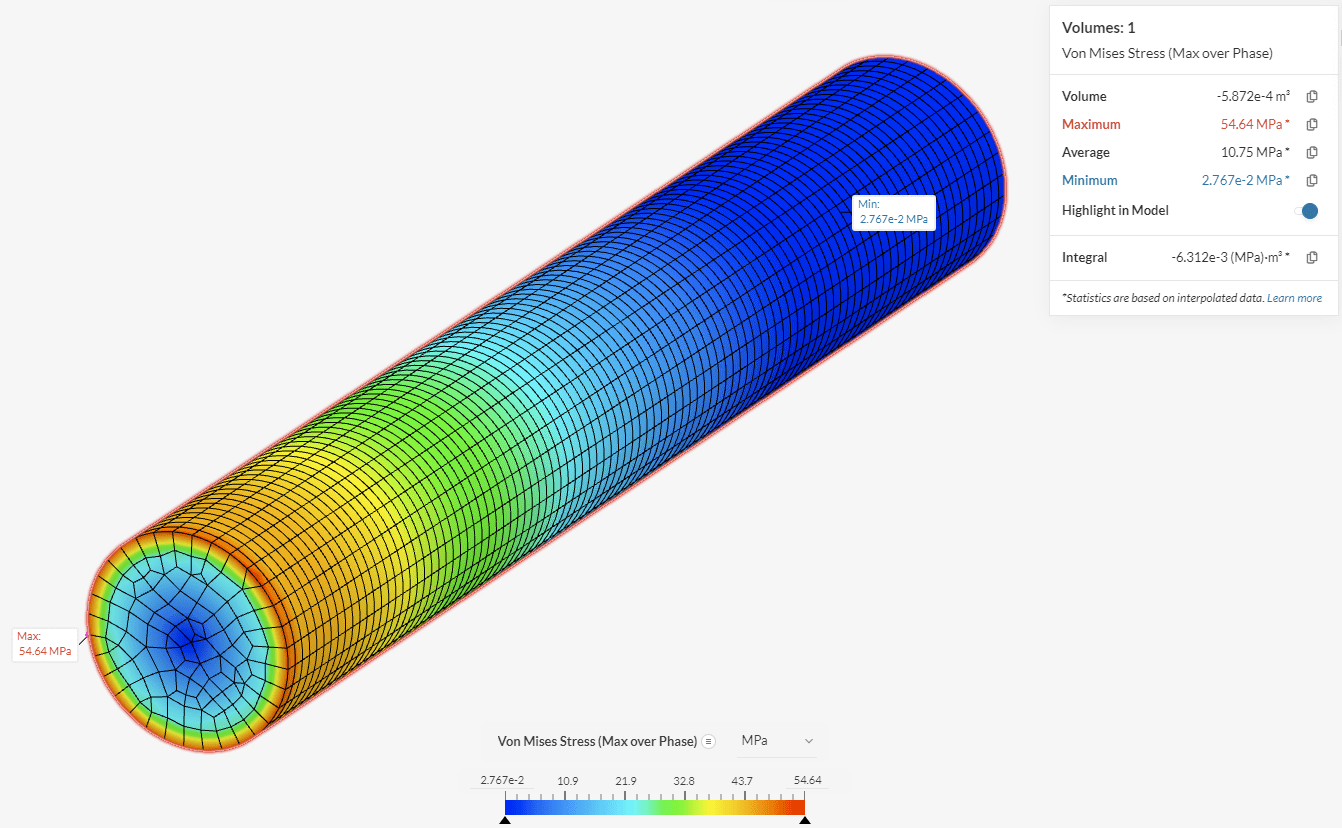
Maximum value of Von Mises stress, max over phase = 54.64 MPa
Competitor Software
The same model was implemented in a competitor FEA tool, which also offers the ‘Max Over Phase’ calculation feature. The implemented model has the following statistics:
- Number of nodes = 37,094
- Number of elements = 8 550
- Tetrahedrals = 0
- Hexahedrons (Hex20) = 8,450
- Prisms (Wedge15) = 100
- Pyramids = 0
- Element type = 2nd order
The max over phase distribution shows the same behavior as SimScale, with the following numeral results:
Maximum Von Mises stress, max over phase = 54.599 MPa
Deviation with respect to the SimScale results = 0.08 %
Numerical Verification
By applying the verification methodology at the point reported for the maximum value of the von Mises stress (max over phase), we obtain the following results.
First, we see the phase sweep expansion of the stress components, appreciating the harmonic functions, peak values, phase angles, etc.
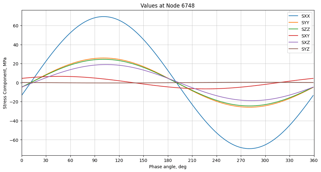
From here, we can compute the history of the von Mises stress by applying the formula at each point of the phase sweep:
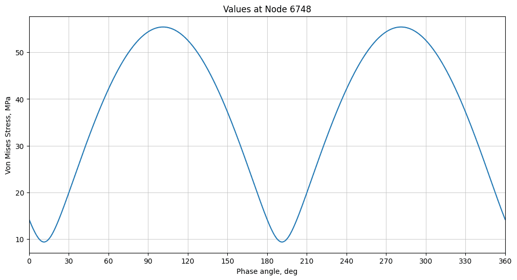
We can appreciate the doubling of the frequency due to the squaring operations in the formula. Examination of the curve yields a maximum value of 55.4335 MPa.
At this same mesh node, the SimScale results show a max over phase value of 54.6369 MPa. The computed deviation at this point is 1.44%.
If we apply the same procedure for all of the mesh nodes in the results, the Normalized Mean Absolute Difference error measurement gives a weighted deviation of 3.9% (here the larger values are emphasized). This error measure is necessary to weigh down the close-to-zero results, for which the relative deviations are always very high.
The NMAD is computed as:
$$ NMAD = 100 \frac{\lt \vert e – p \vert \gt}{max(\lt \vert e \vert \gt, \lt \vert p \vert \gt)} $$
Where:
- The result values from the simulation e
- There reference computed values p
- The average operator (over all the components)
- The absolute value operator |x|
In order to investigate the cause of the discrepancy, we can note that the SimScale methodology is to compute the von Mises stress starting from the principal stresses. Moreover, the principal stresses are computed from a stress tensor formed by the complex stress components.
That is, a complex-valued stress tensor, for which the eigenvalue problem is solved. The result of this computation is a set of three complex eigenvalues that are, in turn, interpreted as the phasor representation of harmonic principal stresses. A phase expansion can be performed for them, for instance.
It is important to emphasize how this methodology assumes that the principal stresses are indeed harmonic functions. Upon further analysis, this does not seem to be a correct assumption, primarily because the eigenvalue computation is not a linear operation on the stress components. Furthermore, a numerical verification is also performed.
In order to test this hypothesis numerically, a comparison was made between the two approaches for computing the phase expansion of the principal stresses:
- “Method A” – This is the method implemented in SimScale, where the principal stresses are assumed to be harmonic functions, and their complex representations are obtained by solving the eigenvalue problem for the complex stress tensor. The phase expansion is then performed on the complex principal stresses.
- “Method B” – This method makes no assumptions about the principal stresses, and works by first obtaining the phase history of the stress components, then forming a real stress tensor at each point in the history. The eigenvalue problem is solved at each point to yield the history of the principal stresses.
The results of the two methods are shown below:
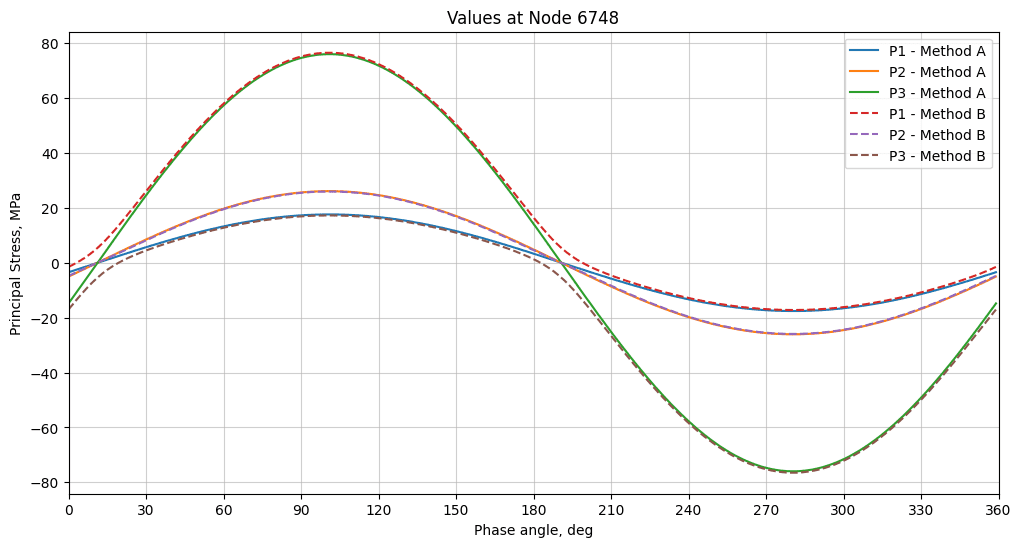
At first glance, it is apparent that the two results are similar. But a closer inspection shows how the actual eigenvalues are not harmonic functions (method B, the dashed lines in the plot), which is expected. The curves are close at the peaks but diverge at the zero crossings.
The real history of the principal stresses seems to be kind of an ‘envelope’ of the assumed harmonic, simplified principal stresses.
Nonetheless, the assumption of the principal stresses as harmonic functions seems to properly capture relevant information, such as the peak values and the phase of max.
Also, it can be seen from the figure that a small deviation is found between each harmonic principal stress and the reference curves (method B). The deviations at the peaks are:
- Deviation in P1 = 0.7%
- Deviation in P2 = 0.5%
- Deviation in P3 = 2.2%
Finally, the von Mises stress computed from method A and B principal stresses are compared, in order to measure the deviations between them:
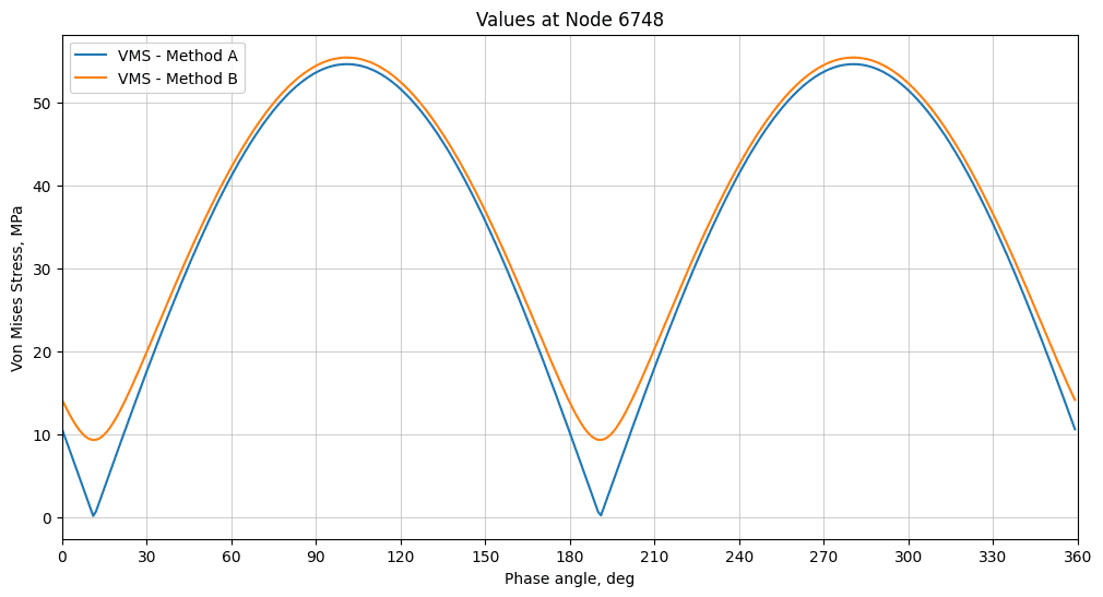
The curves display the same trend, with the phase of max coinciding on both. But the computation of the von Mises stress seems to aggregate the deviations from the computation of the principal stress (aka the assumption of harmonic shape) to showcase a larger deviation.
As related to the results from the analysis of the principal stress methods, the deviations are larger at the valleys and smaller at the peaks.
The values at the peak are:
- VMS max over phase, method A = 54.6369 MPa
- VMS max over phase, method B = 55.4335 MPa
- Deviation = 1.44%
The value for the von Mises stress using method A coincides with the reported results from the SimScale simulation, which confirms that the assumptions and methodologies are correctly captured in this analysis.
The results show that the methodology implemented in SimScale suffers from the limitations of assuming a harmonic shape for the principal stresses and the corresponding impact on the precision of the results. On the other hand, this method is efficient and fast, which offers a profitable tradeoff between computation time and accuracy.
This lack of precision is minimized when the focus of the analysis is to obtain the max over phase, or the peak value of the history because, at this point, the minimum error is expected to happen if the results of this analysis can be generalized. On the same trend, if the interest would shift to deliver the phase sweep history or the minimum values, then the imprecisions of the method would be of greater impact.
Conclusions
A test methodology is presented for the validation of the results given by SimScale’s implementation of the “Von Mises Stress – Max Over Phase” feature.
The methodology works by implementing two alternative ways of computing the max over phase values starting from the harmonic stress components and comparing the final numerical results.
The methodology was implemented on the test case of a round cantilever beam under the action of a rotating bending force. The case was solved using SimScale FEA Harmonic simulation to obtain the stress results.
The comparison of results shows that the SimScale maximum von Mises stress (max over phase) has a deviation of 1.4% with respect to the reference methodology.
The comparison of results with the same model implemented in the competitor software shows a difference of 0.08% in the maximum value, which seems to indicate that a similar methodology is implemented in that product. The qualitative distribution of the results is also comparable.
The computation of the principal stresses was also tested, which revealed that the probable cause of the imprecision in the SimScale methodology lies in the (arguably mistaken) assumption that the principal stresses are harmonic functions.
It is also found that, although imprecise, the SimScale methodology is fast and resource-efficient. It properly captures information such as the “phase of max” and a close “max over phase”, with an error of 1.4% on the peak value of the von Mises stress and of 2.2% on the peak value of the third principal stress.