Modeling Inelasticity With SimScale: Plasticity and Creep
written by
Ajay Harish
updated on
March 26th, 2026
approx reading time
8 Minute Read
BlogFEAModeling Inelasticity With SimScale: Plasticity and Creep
The simplest form of analysis in solid mechanics is linear static analysis. Here, the deformations in the material are assumed to be small, and Hooke’s law (or the linear relation between stress and strain) can be assumed. However, as the load increases, the material behavior (also known as the stress-strain relationship) becomes nonlinear, demonstrating effects like plasticity and creep.
There are several types of nonlinearities, such as material, geometric, and boundary nonlinearities. Thin structures undergo large rotations and displacements in spite of the material satisfying Hooke’s law; these are known as geometric nonlinearities. Alternatively, when certain aspects of the contact phenomenon are involved, nonlinearity exists in the boundary conditions. However, the most common type of nonlinearity is the material nonlinearity observed as a result of the nonlinearity in the stress-strain behavior.
The most challenging problems are, of course, those involving a combination of the above-mentioned nonlinearities and possibly others. For example, in a car crash simulation, the displacements are large and the stress-strain behavior is nonlinear. Additionally, inertia and contact (for example, with other bodies and self-contact) must be considered during the simulation.
In this article, we will discuss the fundamentals of plasticity and creep. For a broader overview of all nonlinear material model types — including hyperelastic and damage models — see our guide to nonlinear material models in FEA.
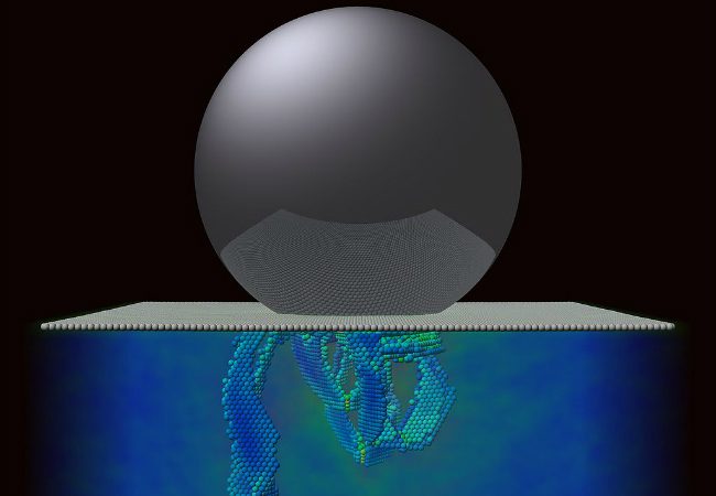
Figure 1: By Gerolf Ziegenhain (Own work) [CC BY 3.0], via Wikimedia Commons
Material Nonlinearity: Plasticity
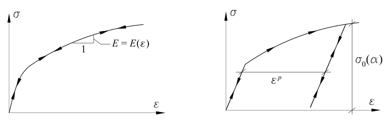
Material nonlinearity is related to aspects of nonlinear elasticity and inelastic phenomena like plasticity, creep, and others. At the point of small stresses, both materials follow a linear stress-strain behavior. Upon an increase in stress, the stress-strain relation is nonlinear, but there is no distinction made between loading and unloading, except for the sign in nonlinear elastic materials. Upon complete unloading, no residual strains are observed.
In contrast, in elastoplastic materials, as the stress increases beyond a threshold (known as yield limit), the stress-strain behavior becomes increasingly nonlinear. Upon unloading, the elastoplastic material leads to a new branch of the stress-strain curve where the material behaves like elastic again. However, upon complete unloading, a residual strain (known as plastic strain) remains. This is described as plasticity behavior observed in the material.
Figure 2: Stress-strain curves for nonlinear elastic material (left) and elastoplastic material (right)
In reality, the curved part observed in elastoplastic materials is quite complicated. For this reason, a number of approximations—known as hardening models—are made to describe this region. There are several models that can be applied to large-scale simulations to replicate the plastic effect. The most common hardening rules are isotropic, kinematic, and mixed. Several complicated hardening rules and plasticity models have evolved over the recent decades. Nevertheless, it is important to understand the physical cause that leads to plasticity, and this varies according to the material. For example, when existing in metals, it is the movement of dislocations, while in polymers, it is due to chain rearrangements.
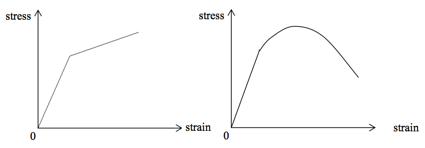
In the presence of hardening, both the elastic and plastic strain continuously increase beyond the yield limit. In other words, the strains increase corresponding with the increasing stresses but at a lower rate than below the yield limit. Surprisingly, in the presence of softening effects, the strains still continue to increase despite a decrease in stress. The difference between hardening and softening is illustrated in Figure 3.
Figure 3: Strain-stress behavior with strain hardening (left) and softening (right)
As shown in Figure 3, strain hardening is demonstrated through a linear hardening model where strains increase with increasing stresses—though at a lower rate than below the yield point. In contrast, strain softening shows that strains continue to increase even when stresses are decreasing.
SimScale’s CEO David Heiny tests the capabilities of the platform to solve a real-life engineering problem. Fill in the form and watch this free webinar to learn more!
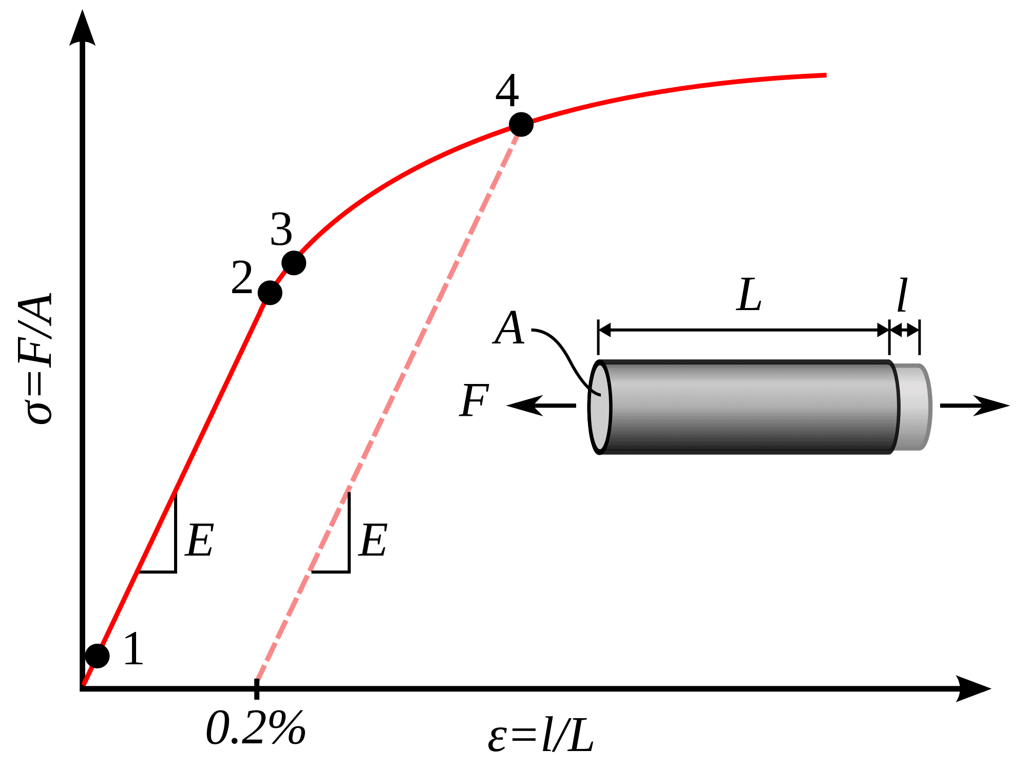
Consider a ductile material being subjected to a uniaxial tensile loading. As shown in Figure 4, as the load increases from Pt. 1 to Pt. 2, the material behaves in an elastic manner. In other words, upon unloading, the material follows the same stress-strain curve it followed during loading.
Figure 4: Typical stress-strain curve obtained during uniaxial tensile testing of ductile material
However, upon loading beyond Pt. 2, the material no longer behaves elastically. In other words, it follows a different path upon unloading. This is shown as unloading from Pt. 4. The point at which the material becomes inelastic is termed as the “Yield Point” and the corresponding stress as “Yield Stress”.
Principal Stresses
At any point, the stress is a symmetric second-order tensor or is represented by a symmetric matrix. This implies that there are six independent values. These stresses are defined in the global coordinate system. Now, if a different coordinate system is selected, the stresses need to be transformed using a transformation matrix.
If a transformation matrix is defined such that the resulting stress matrix is diagonal, then the diagonal elements are the principal stresses. The three columns define the three vectors that form the new coordinate system.
The physical meaning is that the three planes on which these three vectors are normals are only subject to tensile loading—and not shear. The three principal stresses provide the tensile loads on the three planes.
Von Mises Stress
As we have already discussed, the stress tensor has six independent values. However, as previously demonstrated, only one yield stress value is obtained for a material. The question now becomes how to choose which stress value needs to be compared with the yield stress to determine if the material has yielded.
In this case, the uniaxial tensile loading was simple and can be treated as a one-dimensional problem. In this instance, only the stress along the axis of loading can be considered for comparison, but this does not hold true in a general case.
There are several criteria—which are available in literature—that can be used as a comparison with the yield stress. SimScale uses the von Mises yield condition. The von Mises stress can be expressed in terms of the stress tensor components as:
This von Mises stress is used as a comparison to check if the material has yielded. If the von Mises stress is larger than the yield stress, then the material can be said to have yielded.
Linear Hardening: Plasticity
SimScale offers the usage of isotropic hardening rules to describe plastic effects. Linear hardening means that beyond the yield point, the stress-strain relation is still linear. However, the modulus for loading is different from that of unloading.
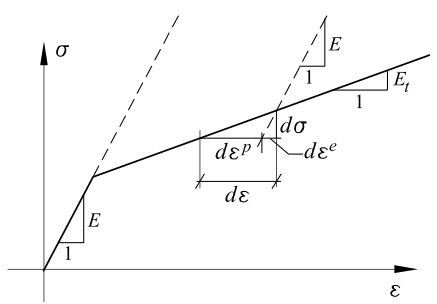
As shown in Figure 5, the slope of the stress-strain curve beyond the yield limit is still positive, but it is still less than the original.
Figure 5: Material demonstrating linear hardening beyond the yield point
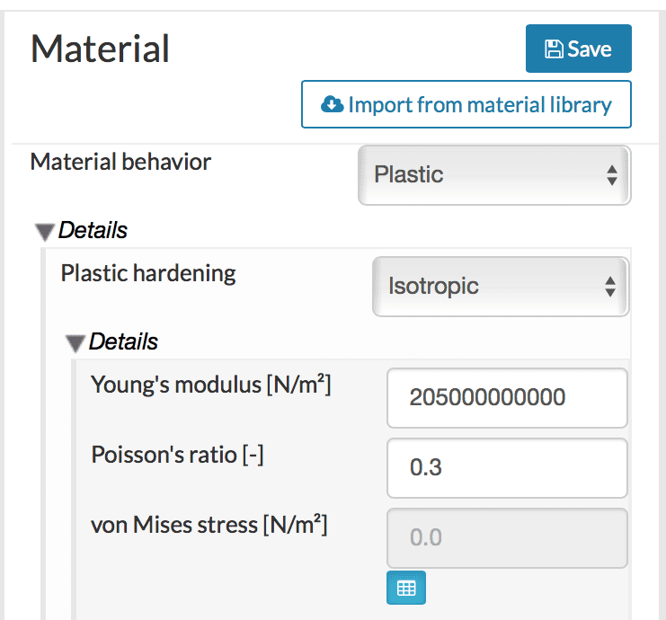
SimScale allows for a modeling plastic effect using the linear hardening model. As illustrated in Figure 6, the inputs are Young’s modulus, Poisson ratio, and von Mises stress, or the yield limit. The yield limit can also be provided through the input of experimental stress-strain data, which is explained in more detail in the SimScale documentation.
Figure 6: Input for plastic material on the SimScale platform
Johnson-Cook Plasticity Model
The Johnson-Cook model is an essential tool for simulating material behavior under extreme conditions, particularly for metallic materials experiencing substantial deformation, high strain rates, and elevated temperatures. It’s particularly useful in finite element analysis (FEA) for predicting how materials will behave under dynamic loading conditions, such as in automotive or aerospace applications.
Key Components of the Johnson-Cook Model
Strain Hardening: The model accounts for the increase in material strength as it deforms.
Strain Rate Sensitivity: It incorporates the rate at which the material is deformed, making it ideal for high-speed impact simulations.
Thermal Softening: The model adjusts for temperature effects, critical in scenarios where materials experience significant heating during deformation.
Due to its ability to predict material behavior under extreme conditions, the Johnson-Cook model is widely used in industries where safety and performance under stress are critical. This includes the design and testing of automotive components, protective gear, and aerospace structures.
Johnson-Cook Model Equation
This model is defined by the following flow stress equation:
$$ \sigma = (A + B\epsilon_{pl}^n)(1+C \log(\overline{\dot{\epsilon}}))(1-\overline T^m) $$
Where:
\(\sigma\) is the equivalent stress.
\(\epsilon_{pl}\) is the equivalent plastic strain.
\(\overline{\dot{\epsilon}} = \frac{\dot{\epsilon}}{\dot{\epsilon}_{ref}}\) is the dimensionless strain rate, with \(\dot{\epsilon}_{ref}\) as the reference strain rate, , usually representing a quasi-static process.
\(\overline T = \frac{T-T_{ref}}{T_m – T_{ref}}\) is the homologous temperature, where \(T\) is the deformation temperature, \(T_{ref}\) is the reference temperature, usually represented by the room temperature, and \(T_m\) is the material’s melting temperature.
The constants in the equation are:
\(A\): Initial yield stress under reference conditions
\(B\): Strain hardening coefficient
\(n\): Strain hardening exponent
\(C\): Strain rate hardening coefficient
\(m\): Thermal softening exponent
The equation can be divided into three key components:
The strain hardening term \((A + B\epsilon_{pl}^n)\) accounts for the increase in material strength with plastic deformation.
The strain rate strengthening term \((1+C \log(\overline{\dot{\epsilon}}))\) captures the effect of strain rate, making the model suitable for dynamic scenarios.
The thermal softening term \((1-\overline T^m)\) adjusts the material’s strength under elevated temperatures.
These components collectively influence the material’s flow stress, allowing for a comprehensive understanding of how materials behave across a spectrum of complex conditions, including those involving significant deformation, high strain rates, and elevated temperatures.
Flexibility of the Johnson-Cook Model
One of the model’s key advantages is its adaptability. Users can apply just the strain hardening term if only plastic deformation needs to be modeled. Alternatively, users can combine all three terms—strain hardening, strain rate strengthening, and thermal softening—depending on the specific material behavior and simulation conditions.
In SimScale, this model can be implemented by inputting the material constants \(A\), \(B\), \(n\), \(C\), and \(m\) fitting to experimental data or literature. This allows for robust simulation predictions involving dynamic loading conditions, elevated temperatures, and high strain rates.
Benefits of Using the Johnson-Cook Model in SimScale
High Accuracy: The Johnson-Cook model offers precise predictions in scenarios where traditional models may fall short, particularly under high strain rates and temperatures.
Versatility: It can be applied across various industries, from automotive testing to aerospace component analysis.
Ease of Use: Despite its ability to model complex deformation mechanisms, SimScale’s interface allows for straightforward implementation of the Johnson-Cook model, with clear guidance on parameter input and model configuration.
Material Nonlinearity: Creep
Creep deformation is a time-dependent deformation. When a constant stress (or force) is applied, the strain initially reaches a particular level. Later on in the process, if the stress is continued to be applied, the strain gradually increases. This happens in spite of the constant force/stress. Such behavior is irreversible and more commonly observed in viscoelastic materials like rubbers and polymeric materials. Creep is not necessarily a damaging phenomenon. For example, creep in concrete allows for reduction of tensile stresses which could have otherwise led to cracks and fracture.
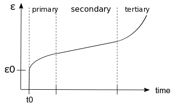
Figure 7: Typical strain behavior of a viscoelastic material over time
As shown in Figure 7, there are three distinct stages of creep. The primary stage demonstrates an initiation of the creeping process and is relatively slow. In contrast, the tertiary stage indicates the formation of necking and is considerably rapid. The secondary stage is when the material undergoes deformation in a reasonably stable manner and is well understood. SimScale facilitates creep deformation in the primary and secondary stages.
As observed above, to simulate creep phenomenon, a relation needs to be defined regarding how the strains change with time and stress applied. Several phenomenon-based models have been defined on the SimScale platform.
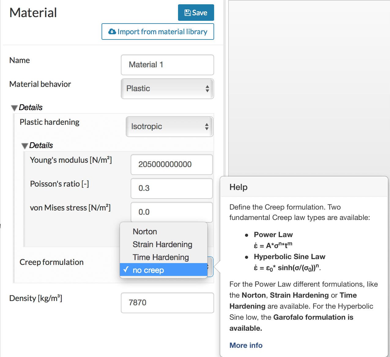
Figure 8: Options provided by SimScale for creep behavior modeling
As demonstrated, all the formulations are equally stable. However, choosing the appropriate law depends on the availability of experimental results and which of the required parameters can be obtained.
Norton is the simplest and depends only on the stress. With Norton, the power law is considered with m = 0, or the dependence on time is not considered.
Time hardening uses the power law with dependence on both the stress and time considered, as shown in Figure 8.
Strain hardening is more complicated. In addition to dependence on stresses, an additional dependence of “creep strain” is also considered as:
$$ \dot{\epsilon}^c = A \times \sigma^n \times (\epsilon^c)^m $$
For more information on the additive decomposition of strains into elastic, plastic, creep, parts, etc. are discussed in more detail in the SimScale documentation.
Conclusion
Overall, SimScale allows modeling plastic and creep effects that are commonly observed in metals, polymers, rubber materials, etc. Each of these options already provides an excellent first-order approximation for modeling these phenomena in a wide variety of materials.
Discover all the simulation features provided by SimScale. Download the document below.