Tutorial 2: Incompressible Water Flow Through a Pipe Junction
In this tutorial, we will carry out a fluid flow simulation of water flowing through a pipe junction. The objective is to get insights into the flow field at the junction of the pipe. There are two inlets and one outlet for this configuration. The simulation will show if there is a re-circulation area near the junction and if the design needs to be optimized accordingly.
The tutorial project “Tutorial 2: Pipe junction flow” has been imported and is open in your SimScale Workbench.
1. Creating a Flow Region
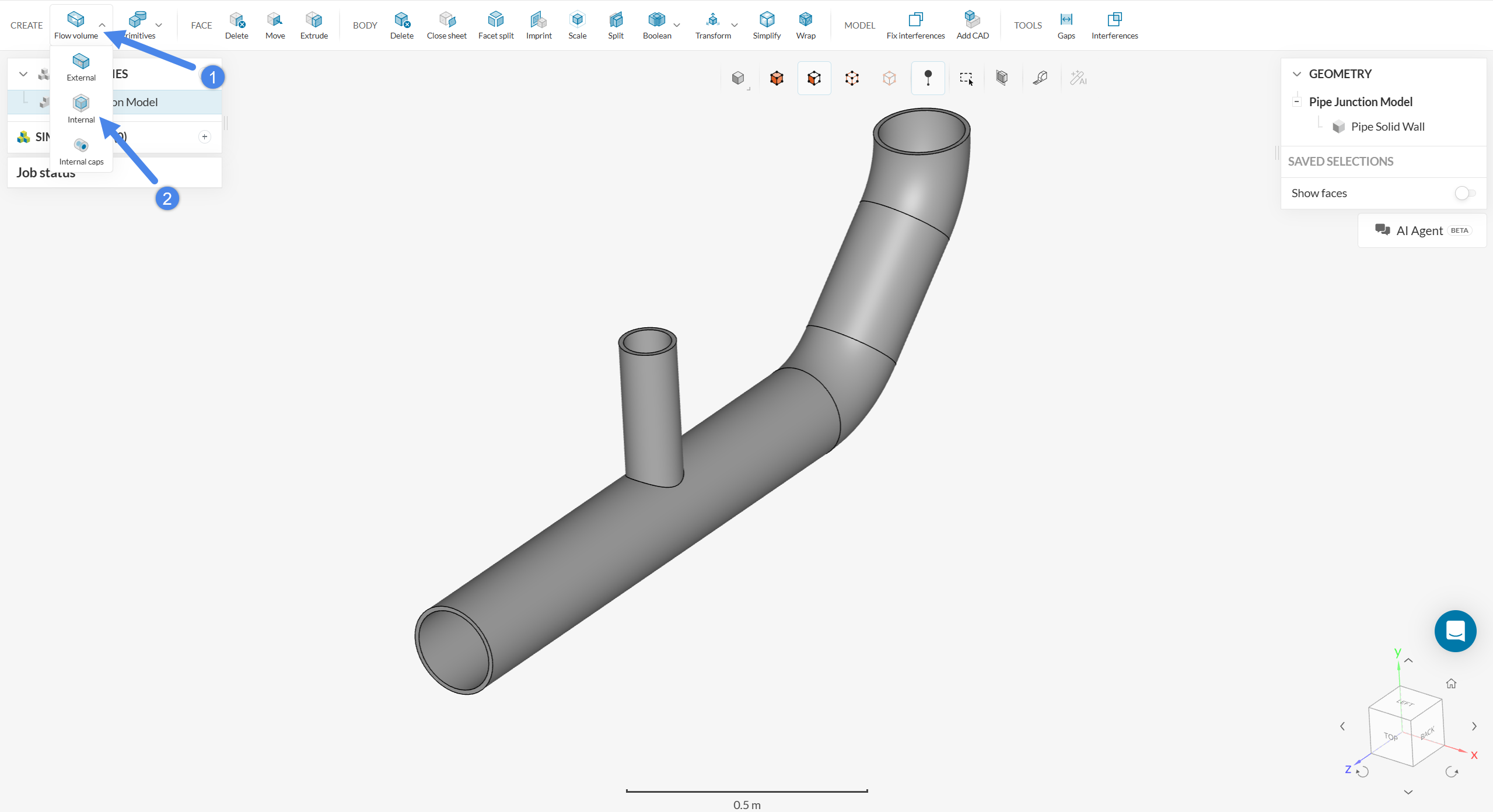
The initial CAD model contains the solid walls of the pipe but not the volume occupied by water. As such, before setting up the simulation, a Flow region, representing the fluid domain, needs to be created.
Since the flow region is internal to the pipe, select an ‘Internal’ flow volume operation:
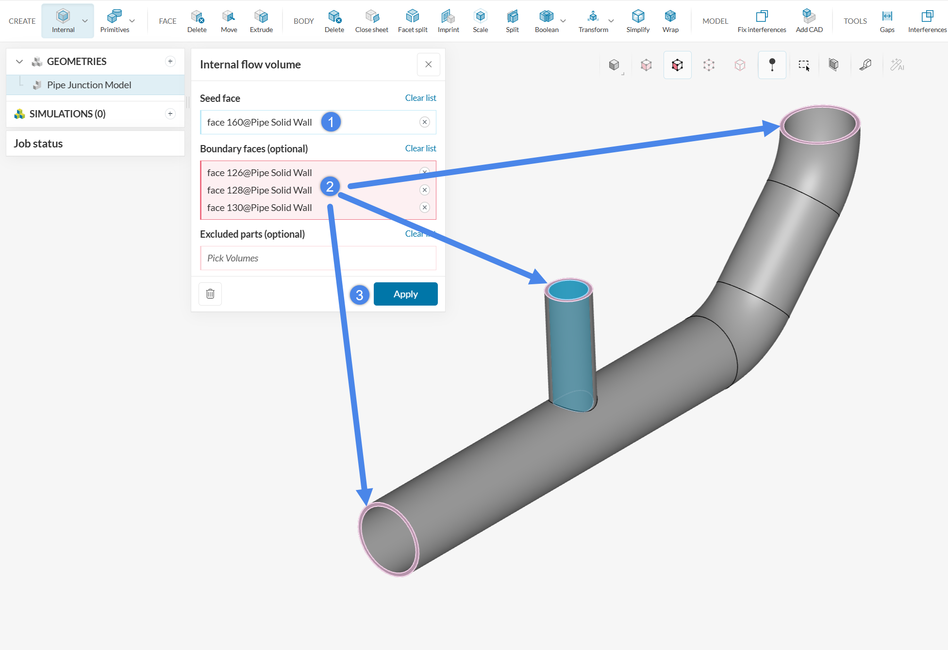
In the internal flow region setup window, seed and boundary faces have to be assigned for this model. Since the tube has 3 openings, there will be 3 boundary faces in pink, below. The boundary faces cover the openings of the tube.
For seed face, only one assignment is needed. It can be any wetted face, so any face in contact with the flow region that we are looking to create works (i.e. a face on the inside of the pipe). Press ‘Apply’ once you assign the faces.
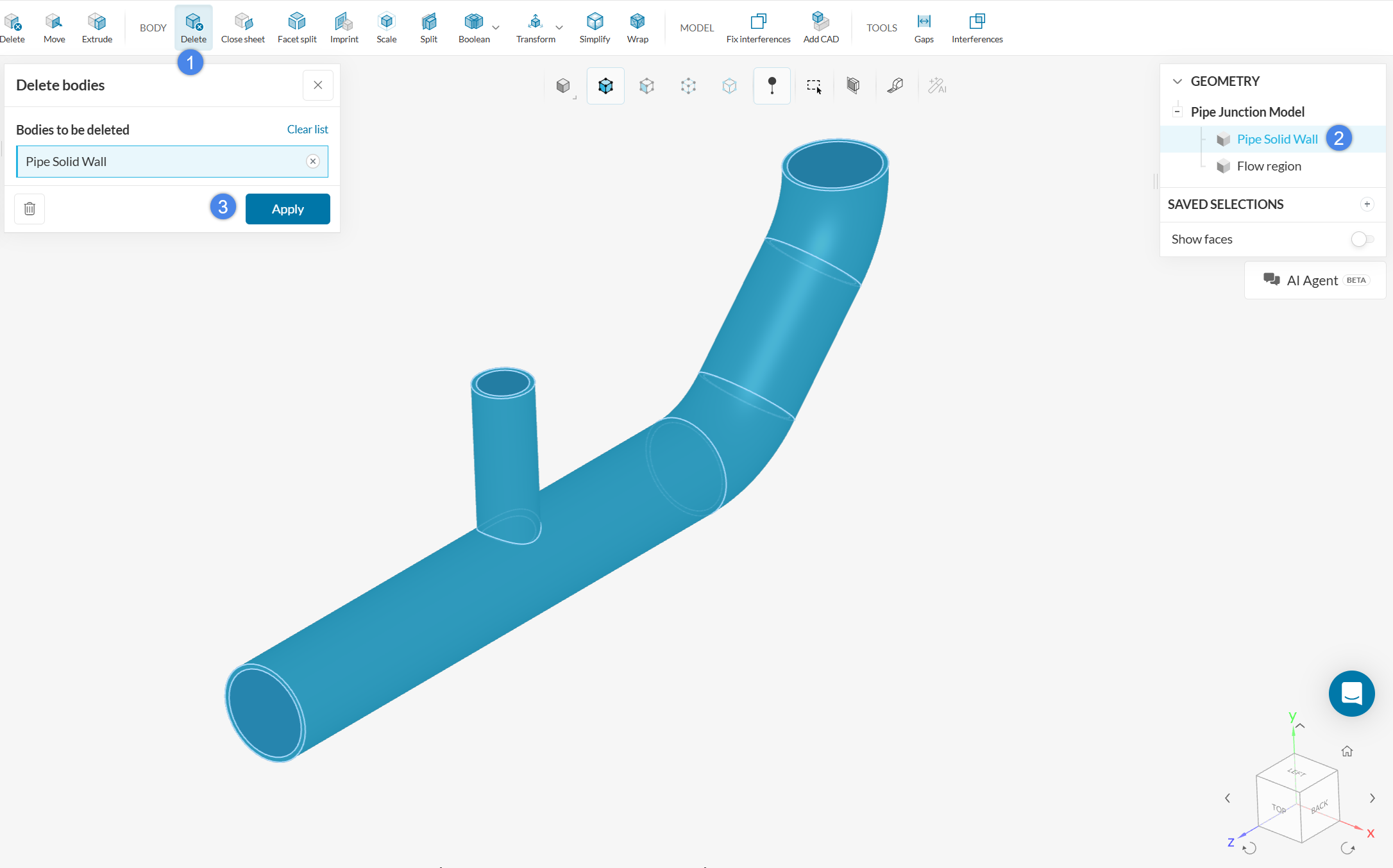
For this type of pipe flow we are only interested in the results within the flow region, so we will delete the solid pipe wall volume before continuing, with a ‘Delete’ body operation:
2. Select the Analysis Type and Create Simulation
You will set up a steady-state flow simulation to obtain an average flow field inside the pipe junction. In the image below, note how the pipe geometry should look like after all CAD operations from the previous section.
At this point, to create a new simulation, select the geometry and click the ‘Create Simulation’ button.
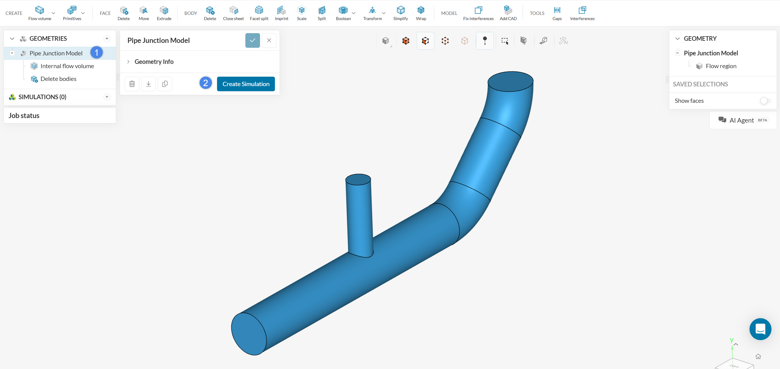
This will open up the Analysis type library. Select ‘Incompressible’ and click ‘Create Simulation’.
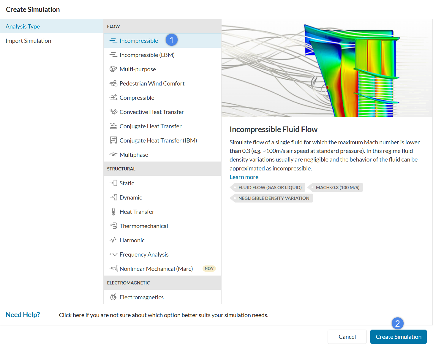
Note
Always choose Incompressible in cases where velocity and temperature gradients are small, independent of your material choice.
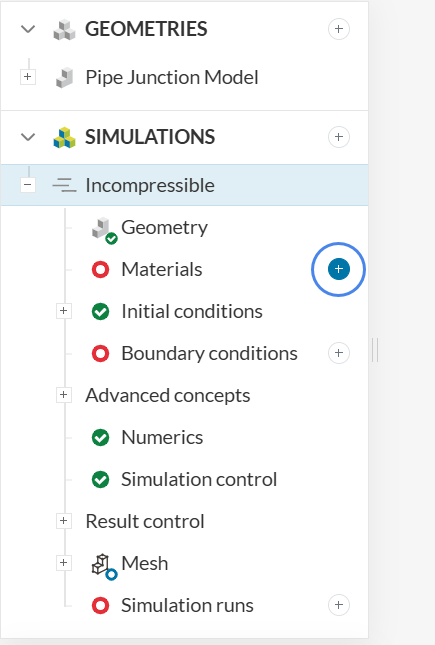
A new simulation tree will automatically be generated on the left side of your screen, containing all the parameters and settings required to run the simulation.
3. Set up the Simulation
A successful simulation setup means a complete and accurate definition of the physics defined within the simulation tree.
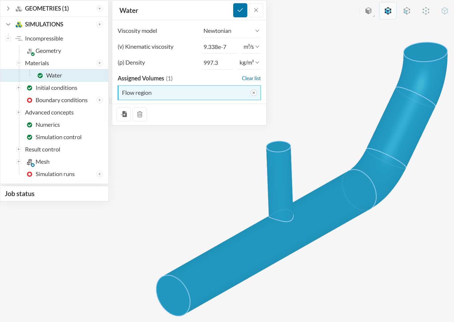
3.1 Material
To assign a new material, click on the ‘+’ button next to Materials in the simulation tree.
This will open the Material library which contains all the available materials for a simulation. Scroll down to select ‘Water’ and click ‘Apply’.
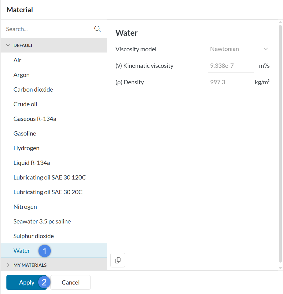
Water will be automatically assigned to the pipe volume.
Note
Note: The color blue indicates that you are in assignment mode.
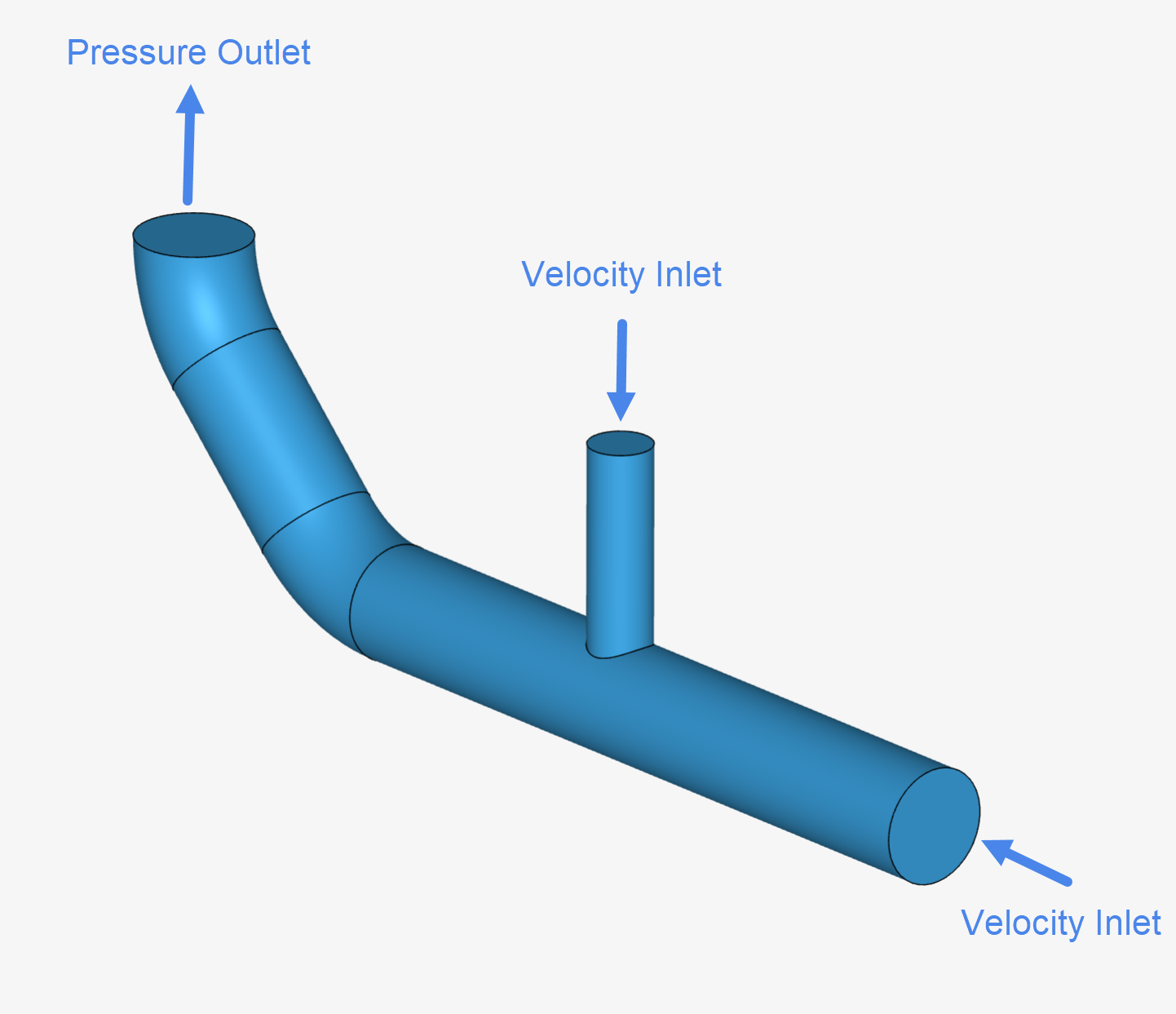
3.2 Boundary Conditions
Boundary conditions are constraints that define the physical boundaries of the simulation, such as the input and output of a pipe. For this simulation, three boundary conditions (Velocity inlet 1, Velocity inlet 2, and Pressure outlet 3) will be necessary so that we can model water meeting at the junction of the pipe coming from the horizontal and vertical inlets.
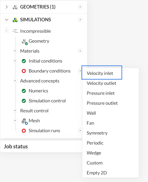
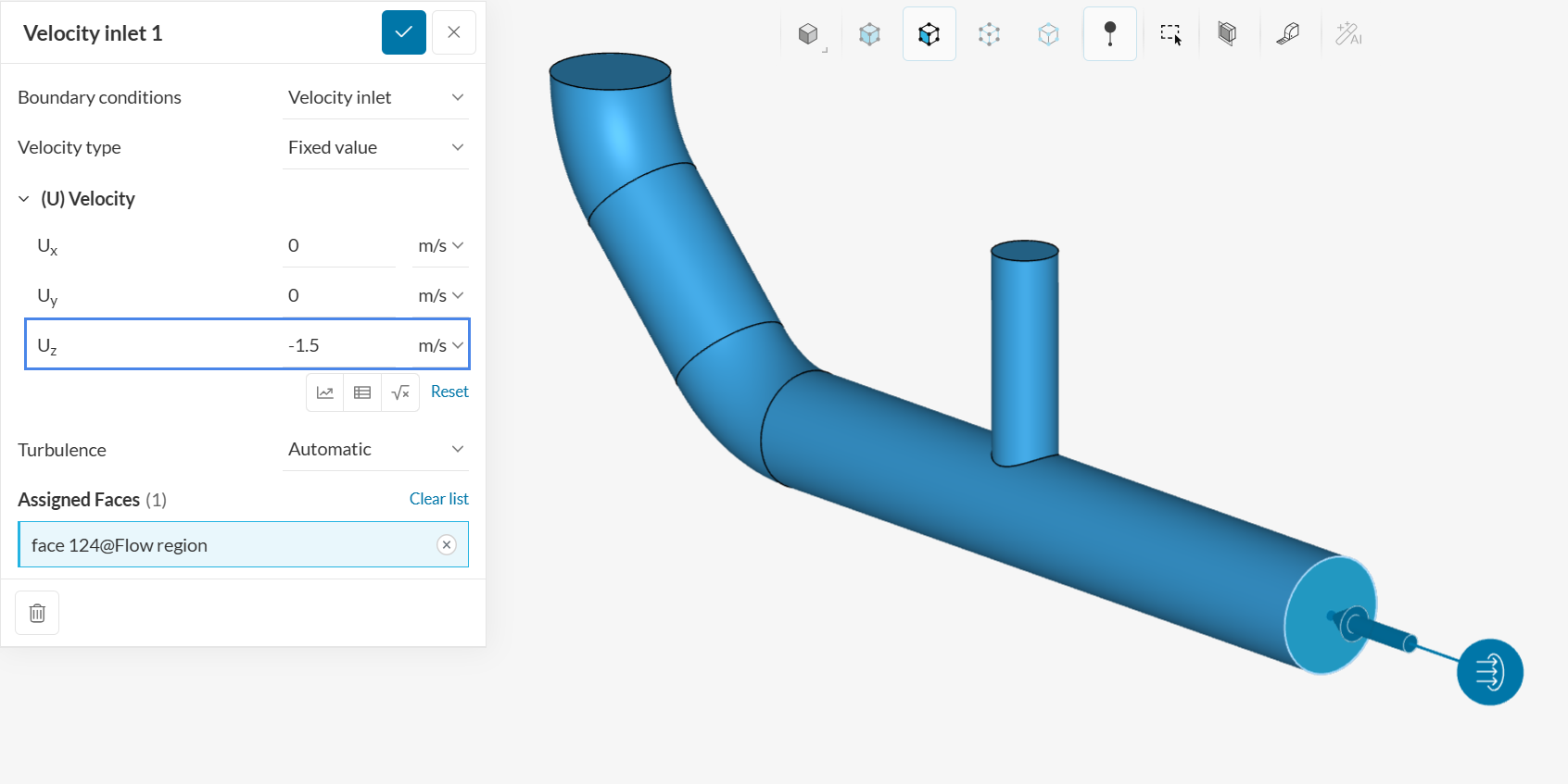
A. Velocity Inlet 1
To create a new boundary condition, click on the ‘+’ button next to Boundary conditions in the simulation tree. Select ‘Velocity inlet’ from the list.
Set the velocity in z-direction to ‘-1.5’ \(m/s\). This will assign a flow with the specified velocity to the assigned face. In this case, flow from the negative z-direction is needed to model the horizontal flow. The global coordinates can be found in the viewing cube at the bottom right of your screen.
Select the horizontal face in the viewer. This will assign the face as a velocity inlet.
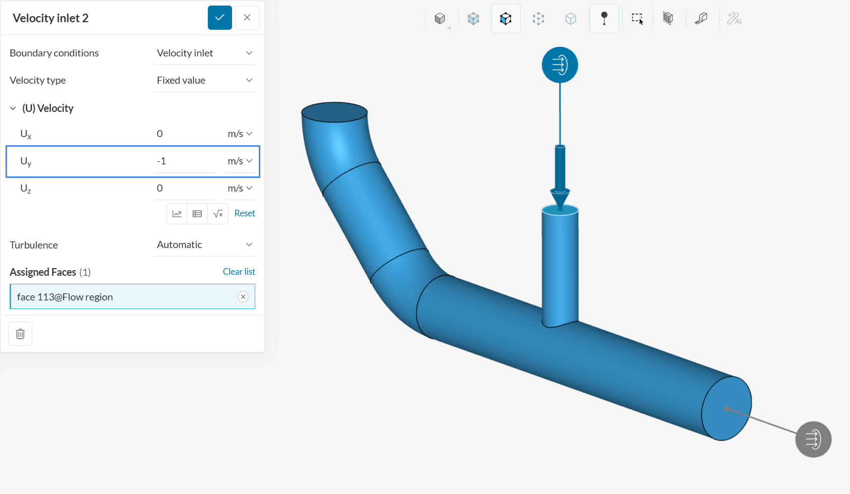
B. Velocity Inlet 2
We will set up another velocity inlet to simulate a vertical flow by following the same steps as before. Set the velocity in y-direction to ‘-1’ m/s. Select the face to assign the new velocity inlet.
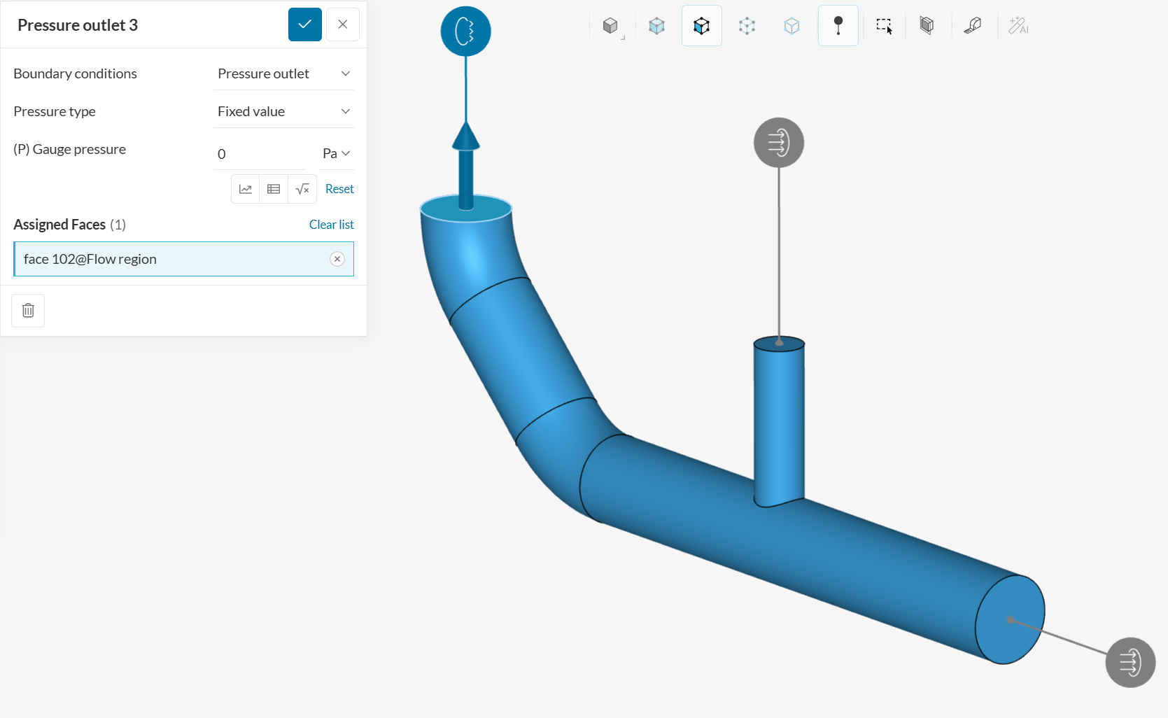
C. Pressure outlet
Last but not least, we will add a third boundary condition which is the ‘Pressure outlet’. Select the face to assign it as a pressure outlet boundary condition.
Note
The color turns blue, indicating that they will be assigned to the current boundary condition.
4. Start the Simulation
Now you are ready to start your simulation run.
The Numerics, Simulation Control, and Mesh settings are set by default and do not have to be changed for this simulation.
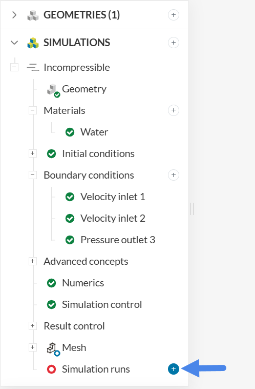
Create a simulation run by clicking on the ‘+’ button next to Simulation runs in the simulation tree.
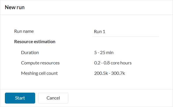
A dialog box will appear stating the estimated amount of resource consumption. Click ‘Start’ in the New run dialog box to start the simulation run.
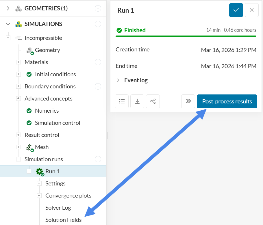
Once the simulation run is finished, the status will be changed to Finished in the run settings panel.
5. Post-Processing
Click ‘Post-process results’ or ‘Solution Fields’ under the run to open the post-processor. SimScale’s integrated post-processor consists of filters and different viewing tools to better visualize and download the simulation results.
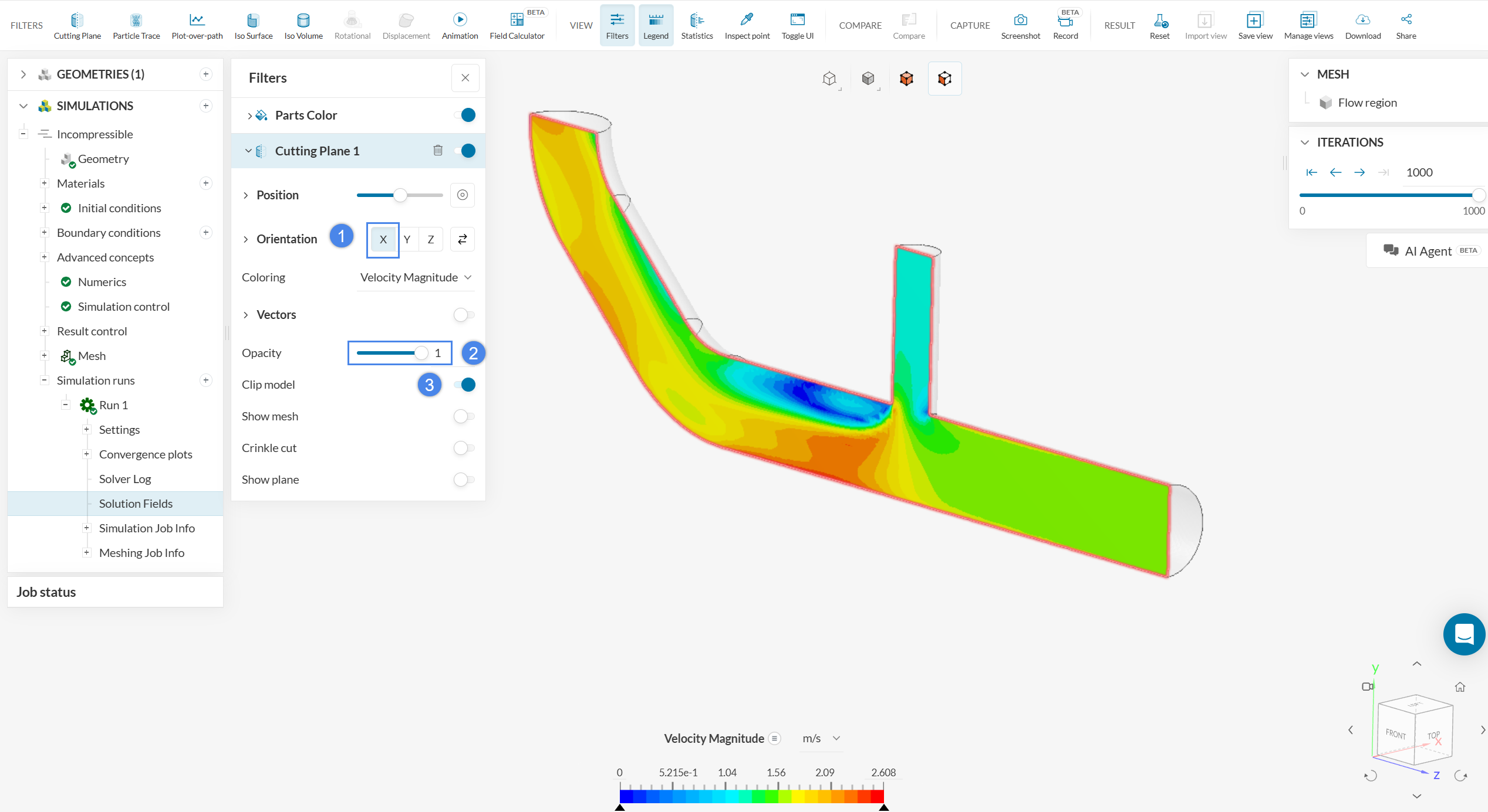
After opening the post-processor, a cutting plane will be automatically applied. Now, we want to show the flow inside the pipe. Therefore, we will change the orientation of the plane to the x-axis by clicking on ‘X’ besides Orientation. Also, make the cutting plane fully opaque by setting the Opacity to ‘1’, and enable Clip model.
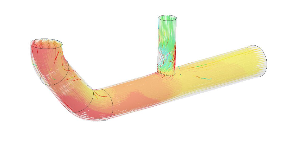
You can also find areas where re-circulation occurs by visualizing the velocity vectors as shown below. Turn on the toggle beside Vectors to show the velocity vectors. Next, to make the vectors more clear, you can set the color of the vectors to black beside Coloring.
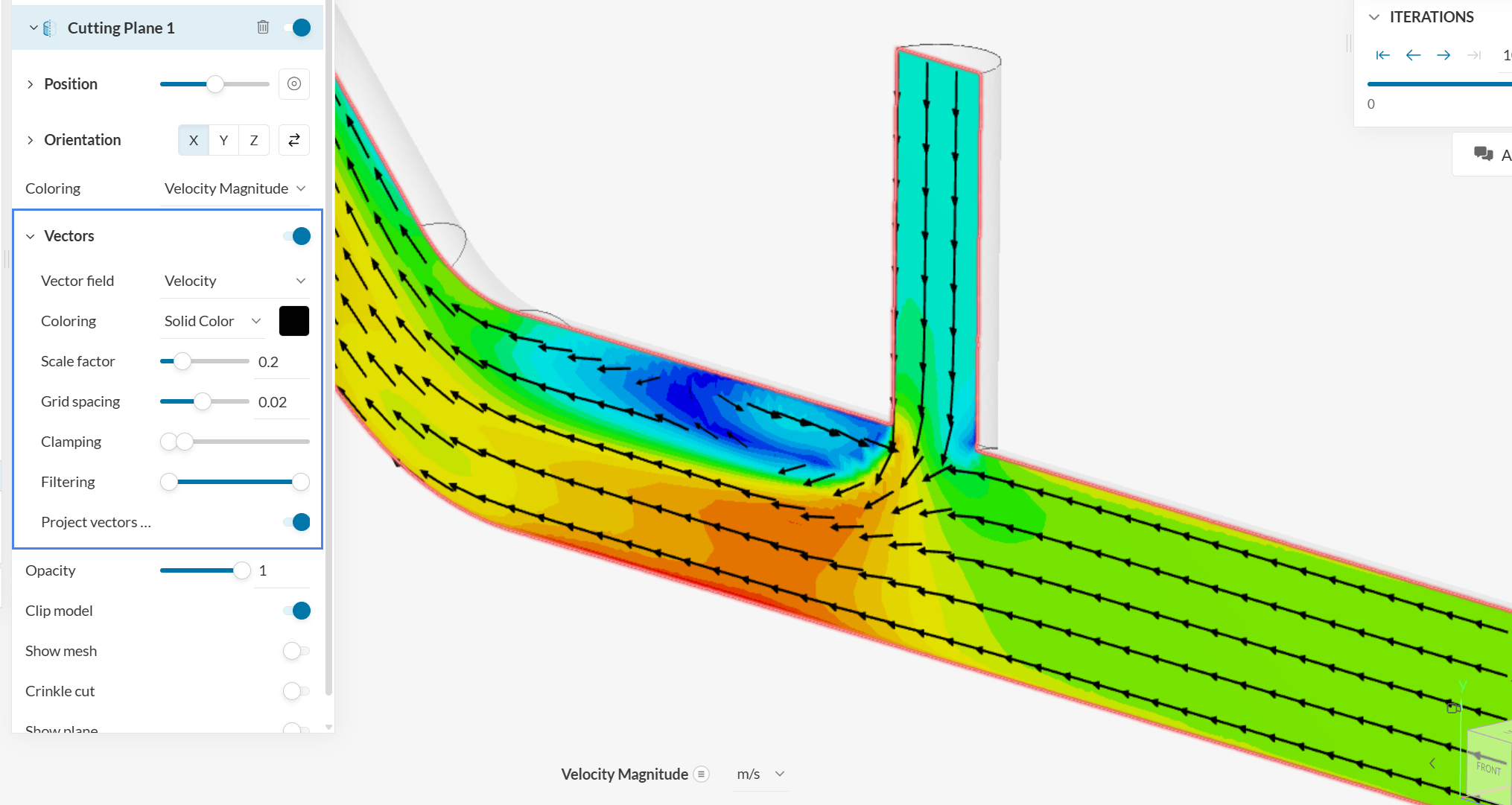
Based on the velocity vectors, we can see a large re-circulation region in the areas near the junction, so this is a region that may require some improvements.
Congratulations! You just finished your first internal fluid flow simulation on SimScale!
Find more tutorials on our website: SimScale Tutorials and User Guide