Hello @babissak12 , this is a great question that has a very detailed answer. Besides our answers here, I’d also recommend you to review the literature with keywords: RANS, turbulence models, eddy viscosity, eddies, DNS, LES.
Turbulent (Eddy) viscosity is an artificial term used in Reynolds Averaged Navier Stokes (RANS) equations to account for the reduction in turbulent due to rotational effects (vortices). As the name suggest, RANS equations are time-averaged equations that should be used when you don’t need instantaneous properties of the flow.
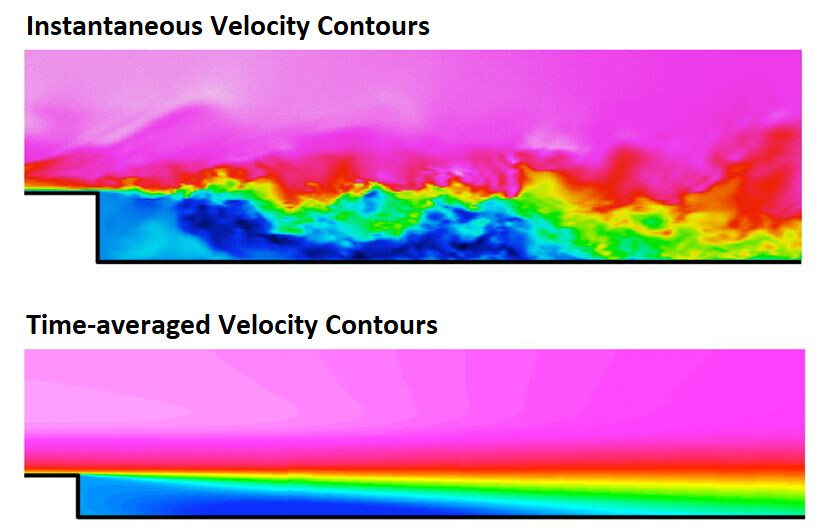
As you’ll see on the figure above, RANS (time-averaged velocity contours) tends to model the turbulence(chaotic flow) instead of simulating it, which is usually done in LES and DNS approaches. To compansate the reduction in turbulent flows influence, an artificial diffusion term is produced by the turbulence models: Turbulent (Eddy) viscosity.
But how can we take advantage of turbulent viscosity contours in our solution field? We would expect this artificial diffusion term to be significantly higher than molecular viscosity within the turbulent region. (Molecular viscosity is a fluid property, not a flow property and it’s defined under Materials in the platform) Hence, regions with higher values of turbulent viscosity will indicate a turbulent/chaotic flow.
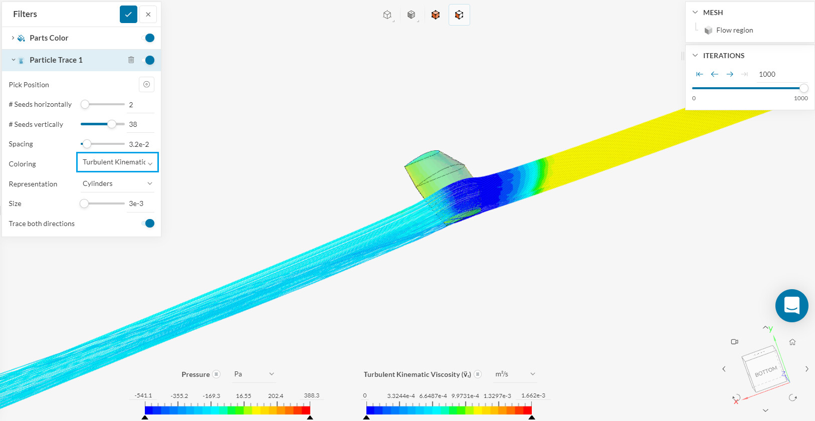
In your solution field you’ll see that there is a region far from the wing wall that almost has a constant turbulent kinematic viscosity. Turbulent viscosity within freestream region is calculated based on the turbulent kinetic energy and specific dissipation rates defined in boundaries. (In this case it’s defined by using the inital conditions when a velocity inlet boundary condition is used) Turbulence models will have no influence on the turbulent viscosity within the freestream region since they are only activated at a finite difference downstream of the walls. In case you want to learn more about initial values of turbulent quantities, here is a detailed post on the Forum which may be helpful.
Turbulent viscosity production by the turbulence models becomes important near the walls. Near laminar regions (around the leading edge of the wing), you’ll observe that production of turbulent viscosity, consequently turbulent viscosity value, is relatively lower because the flow is still smooth and regular. Once the flow becomes chaotic and turbulent (near the trailing edge of the wing), you’ll observe a significant increase in turbulent viscosity produced by the turbulence model.
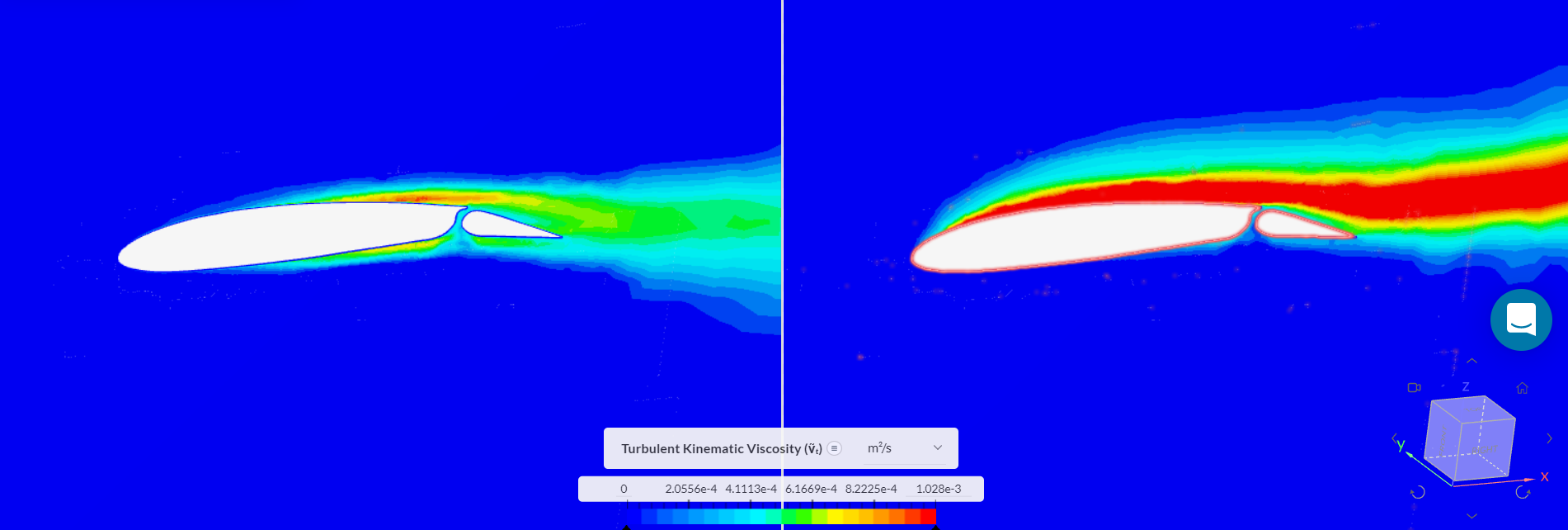
Looking at another application by using the compare tool, here a wing configuration is simulated in two different angle of attacks (0 and 10 degrees).
0 degrees of angle of attack (left) and 10 degrees of angle of attack (right)
By looking at the turbulent viscosity contours here, I can infer that:
-There is an almost laminar region in both cases near the leading edge of the airfoil that is understood by the small values of turbulent viscosity,
-Flow is highly turbulent, unpredictable due to forming of vortices on the upper side of the airfoil in case of 10 degrees of angle of attack,
-In both cases, turbulent viscosity values are higher on the upper side of the airfoil than the lower side because the flow speed is higher on the upper side. Increase in flow speed → Increase in turbulence.
-I like that turbulent viscosity values are relatively low on the upper side of flap surface. This proves that the slotted flaps are actually doing their job by compansating the boundary layer seperation on the upper surface of the flap.
In general, it’s completely up to you how you plot the contours. In this case I would prefer cutting planes and vectors to examine flow seperation near trailing edges. In case you plot turbulent viscosity contours on streamlines, it’s likely that you’ll observe higher values around streamlines with high curvature.
Hope these are helpful,
Kaan.