\underline{\textbf{What is Turbulence?}}
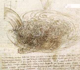
Figure 1: Visualization of a flow by Leonardo Da Vinci
Figure 1 shows one of the first visualizations to study turbulent flows. Those phenomena were called “turbolenza” by Leonardo, who also wrote:
“Observe the motion of the surface of the water, which resembles that of hair, which has two motions, of which one is caused by the weight of the hair, the other by the direction of the curls; thus the water has eddying motions, one part of which is due to the principal current, the other to the random and reverse motion” ^1.
\underline{\textbf{Motivation}}
Almost every flow we meet in engineering applications—no matter if they are pipe flows, flat plate boundary layers, wakes and even more complex three-dimensional flows—become unstable over a certain Reynolds number. At low Reynolds numbers, flows are laminar whereas at higher Reynolds numbers we can observe flows becoming turbulent. The flow develops a state of motion of chaos and randomness in which the pressure as well as the velocity change continuously.
As mentioned, most of the flows of engineering importance are not laminar so there is not only a theoretical interest in turbulence. CFD techniques help to understand and represent the effects and influence of turbulence.
Even though there is a widespread occurrence of turbulent flows and although many of the greatest physicists and engineers of the 19 ^{th} and 20 ^{th} centuries studied this phenomenon, the problem of turbulence remains the last unsolved problem of classical physics and is still not understood in full detail. Remember also that to this day there is a 1 million US dollar prize for proving the Navier-Stokes existence and smoothness problem in \mathbb{R}^3 (Clay Mathematics Institute - Navier-Stokes)
\underline{\textbf{History}}
- Euler (1755):
- Equations for an ideal fluid
- Navier (1822) – major contribution \rightarrow Navier-Stokes Equation (NSE)
- Navier derived the NSE based on a molecular theory
- Viscosity as a function of molecular spacing
- Stokes (1845)– Paper: friction of fluids in motion and the equilibrium and motion of elastic solids
- Publication of a derivation based on Newton’s laws of motion
Until the late 19 ^{th} century there was no substantial progress in understanding turbulence. The cornerstone of most turbulent models was provided by Joseph Valentin Boussinesq and the so-called Boussinesq Approximation. He was also the first one attacking the closure problem by introducing the eddy viscosity.
Boussinesq hypothesis: “turbulent stresses are linearly proportional to mean strain rates”
Experiments of Reynolds around 1894 led to the identification of the so-called “Reynolds number” which states the relation between the inertia forces and viscous forces.
Reynolds was also the one introducing the decomposition of flow variables into a fluctuating part and mean part (“Reynolds Decomposition”).
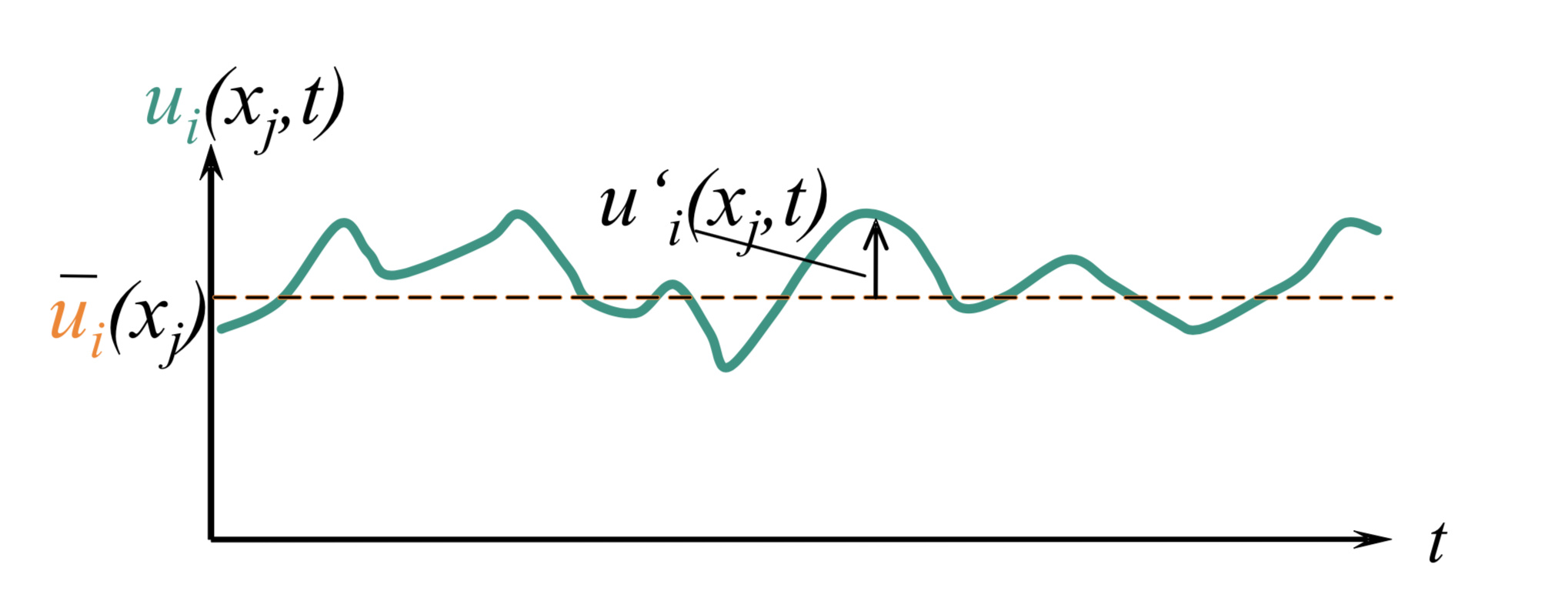
Figure 2: The Reynolds decomposition
- Major result from Prandtl (1925) in predicting the eddy viscosity introduced by Boussinesq. Prandtl’s so-called mixing-length theory was based on the analogy between turbulent eddies and molecules using the kinetic theory in order to determine the length as well as the velocity (time) scales that are necessary to construct eddy viscosity.
The approach by Prandtl has never been used to make meaningful predictions of turbulent flows, yet it does a really good job “postdicting” the behavior of simple flows.
-
G.I. Taylor (1930’s) was the first researcher using advanced mathematical methods. Introducing formal statistical methods involving correlations, Fourier transforms and power spectra.
-
In a paper from 1935, he presents his assumptions that turbulence is a random phenomenon and shows statistical tools for homogeneous, isotropic turbulence.
-
A very valuable contribution by him was his “Taylor hypothesis”, enabling the conversion from temporal data to spatial data.
-
Karman and Howarth (1930s) gave an analytical solution in the limiting isotropic space and introduced the so-called “von Kármán constant”.
-
Leray (1933/34) was the first doing mathematically-rigorous analyses of the Navier-Stokes equations.
-
Kolmogorov (1941) published three papers (results are now referred to as the “K41 theory”) which are ones of the most important and most quoted in turbulence theory.
-
Landau and Hopf (1940s) proposed that as the Reynolds number increases a typical flow undergoes a transition during each an additional frequency arises due to instabilities in the flow, leading to random flow behaviour.
-
The first books on turbulence were published in the 1950s by Batchelor, Townsend, Hinze and others.
-
E. Lorenz (1963) published a paper about machine computations leading to a different way to view turbulence. His work presented a deterministic solution to a simple model of the NSE. This approach could not be distinguished from random approaches. This solution exhibited the feature of sensitivity to initial conditions (“strange attractors”) and showed the nonrepeatability.
-
Throughout the 1960s, progress has been made in the mathematical understandings of the NSE (existence, uniqueness and regularity of solutions)
-
In the late 1950s people like Kraichnan used mathematical methods from quantum field theory to analyze the phenomenon of turbulence and tackle the closure problem (“More-Unknowns-Than-Equations-Problem”). This involved Fourier series, Fourier transformation, Feynman diagrams, etc.
-
Significant progress has been made in the decade of the 60s regarding decay of isotropic turbulence, return to isotropy of homogeneous anisotropic turbulence, boundary layer transitions, etc.
-
Papers by Ruelle and Takens (1971) gave a first insight to “modern” turbulence showing that the NSE (when viewed as a dynamical system) have the potential of producing chaotic solutions being sensitive to inital conditions (SIC) and associated to the strange attractor.
\underline{\textbf{Definition}}
In his book “An Informal Introduction to Turbulence”, A. Tsinober stated that "there is no good definition of turbulence".
One of the “best” definitions of turbulence was formulated by Lewis Fry Richardson:
"Big whorls have little whorls,
which feed on their velocity;
And little whorls have lesser whorls,
And so on to viscosity."
This “poem” about turbulence contains the physical information that energy is injected into the flow on large time and length scales, but the energy undergoes a so-called “cascade” transferring energy successively to smaller scales until the final dissipation (convertion to thermal energy) on a molecular scale (diffusion).
The second physical phenomenon of turbulence covered by Richardson is the dissipation of kinetic energy.
Another definition is by T. von Kármán who quoted G. I. Taylor:
“Turbulence is an irregular motion which in general makes its
appearance in fluids, gaseous or liquid, when they flow past
solid surfaces or even when neighboring streams of the same
fluid flow past or over one another.”
Hinze defined turbulence in the following manner:
"Turbulent fluid motion is an irregular condition of the flow
in which the various quantities show a random variation with
time and space coordinates, so that statistically distinct average
values can be discerned.”
And, in fact, we can see that Tsinober was right in some sense saying that there is no good definition of turbulence because every definition given above does not precisely characterize turbulent flows in the sense of predicting them. And it is not known a priori when turbulence will occur, and what the extent of it will be with which intensity.
G. T. Chapman and M. Tobak described the evolution in terms of three eras:
1. Statistical
2. Structural
3. Deterministic
“Turbulence is any chaotic solution to the 3D Navier–Stokes
equations that is sensitive to initial data and which occurs as
a result of successive instabilities of laminar flows as a bifurcation
parameter is increased through a succession of values.”
This definition is vague and yet contains information that allows a detailed examination of flow states related to turbulence.
-
It specifies the Navier-Stokes equation, which may exhibit turbulent solutions where previous definitions have failed.
-
It requires a chaotic behaviour of the fluid, erratic and irregular as mentioned in earlier definitions, but deterministic and not random (NSE are deterministic) which is in contradiction to Hinze’s definition but supported by experimental data.
-
Turbulence is three-dimensional, which is consistent with classical viewpoints (for instance, Tennekes and Lumley) where the generation of turbulence is described by vortex stretching which can only occur in 3D (there is also 2D turbulence for instance in magnetohydrodynamics).
The modern definition requires a “sensitivity to initial data” which allows us to distinguish irregular laminar motion from what is turbulence. This is directly connected to modern mathematical theories of the NSE implying the already mentioned sensitivity to initial conditions (SIC) which is the hallmark characteristic of the “strange attractor” description of turbulence.
The theory of stability loss of laminar flows has been studied for more than a century (studies of boundary layers). The modern approach includes the bifurcation theory, opening the way to describe dynamical systems through powerful mathematical tools. ^2
Before a small excursus to “deterministic chaos”, we briefly summarize the physical attributes of turbulence:
-
nonrepeatabile (“SIC”)
-
chaotic and random behaviour
-
enhanced diffusion (mixing) and dissipation (on a molecular scale by viscosity)
-
3D, time-dependant and rotationality (\rightarrow potential flow not turbulent since it is irrotational by definition)
-
large range of time and length scales
-
intermittency in space and time
\underline{\textbf{"Deterministic Chaos"}}
Often turbulence is defined as “deterministic chaos”. But what is deterministic chaos and where is the link between two terms having the opposite meaning? It seems to be an oxymoron at first sight. In fact, when talking about something chaotic, we think about randomnesss. And yet, randomness alone is not a sufficient term to describe chaos.
The term deterministic means nothing else than to determine a system’s behaviour for the future (predictability). The question that arises is if even a deterministic system can behave in an erratic manner or be chaotic. Indeed there are systems like the so-called “double pendulum”. The motion and behaviour of such a system are very erratic but still follow certain patterns. The explanation for this has already been mentioned and is the “sensitivity to initial conditions (SIC)”.
Figure 3: The Double Pendulum
\underline{\textbf{Governing Equations and their problems}}
Remember the Millennium Prize problem we addressed in the first part of this article? To be a bit more precise, the problem is to prove that solutions will always exist! The question that follows from this assumption is if my equations, namely the Navier-Stokes Equations (short NSE), can describe arbitrary fluids with arbitrary initial conditions in the future. That seems quite contradictory on what we’vepreviously discussed, when talking about the sensitivity to initial conditions (SIC), right?
Leray has proven in 1934 that there exists at least one global in time finite energy weak solution of the 3D
Navier-Stokes equations. In this paper Tristan Buckmaster & Vlad Vicol prove that weak solutions of the 3D Navier-Stokes equations are not unique in the class of weak solutions with finite kinetic energy. Moreover, they show that Hölder continuous dissipative weak solutions of the 3D Euler equations may be obtained as a strong vanishing viscosity limit of a sequence of finite energy weak solutions of the 3D Navier-Stokes equations. For a beginner, that sounds quite complicated, doesn’t it?
To simplify things a bit more, imagine that you have to prove that a solution of the NSE exists in the first place. As the NSE implies to calculate changes in quantities like the velocity and density, you might run into trouble. Imagine the scenario where you simulate a flow and all of a sudden one particle among all the parcels that exist move infinitely fast. How do you want to calculate the change of an infinite big value? It is impossible and we have a problem what is called “blowup”. This infinitely fast-moving particle might cause that the kinetic energy will grow infinitely high which is simply unphysical behavior—this quantity has to be finite!
\underline{\textbf{Short excursus: Blowup}}

Figure 4: Uniqueness and Non-Uniqueness
\underline{\textbf{Short excursus: How to overcome blowup?}}
One idea to overcome the crux of the matter is to define something called a “weak solution” that you might have heard of, for instance, in the field of the finite element analysis (no? then have a look at this). Instead of calculating every single solution of the field, we just calculate some points in the field and work with approximations.
As mentioned earlier, the French mathematician Jean Leray defined an important class of weak solutions in 1934. Rather than working with exact solution vectors, the so-called “Leray solutions” take the average value of vectors in small neighborhoods of the vector field. Leray proved that it is always possible to solve the NSE when you allow your solutions to take this form and these solutions never blow up.
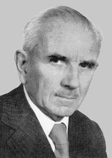
Figure 5: French mathematician Jean Leray
Leray established a new approach to the Navier-Stokes problem: Start with Leray solutions, which you know always exist, and see if you can convert them into smooth solutions, which you want to prove always exist.
\underline{\textbf{Do we win 1 million \$ now?}}
In order to solve the Millennium Prize problem, we have to show that the solutions we created are smooth and unique, which corresponds to a physical behavior that goes only in one way and not end up in two different physical configurations. The two mathematicians from Princeton university, Tristan Buckmaster and Vlad Vicol, consider solutions that are even weaker than Leray solutions. These solutions involve the same averaging principle as Leray solutions but also relax one additional requirement (the so-called “energy inequality”). The method they use is called “convex integration”. ^4
The problem here is that the solutions are nonunique and they give simple examples to understand this non-uniqueness:
-
The water starts still and remains still forever
-
The water starts still, erupts in the middle of the night, then returns to stillness
In the future, researches may work with slightly stronger solutions to get better results or at least see if there are configurations that can not take two configurations from the same initial state.
\underline{\textbf{Related Topics}}
\underline{\textbf{Resources}}
Figure 6
\underline{\textbf{Picture References}}
- Figure 1: \https://www.giss.nasa.gov/research/briefs/canuto_01/
- Figure 2: Jochen Kriegseis - Lecture slides of “Experimental Fluid Mechanics”
- Figure 3: Double Pendulum GIF created with MAPLE 2015
- Figure 4: Quanta Article on Wrinkles of the NSE
- Figure 5: Jean Leray
- Figure 6: Turbulence GIF
\underline{\textbf{Literature References}}
- ^1 Da Vinci Page
- ^2 Introductory Lectures to Turbulence - Physics Mathematics and Modeling by J.M. McDonough
- ^3 Quanta Magazine - NSE
- ^4 Quanta Magazine - Wrinkle in the Famous Equations