Direct Approach
As mentioned in my introduction the Finite-Element-Method consists of the following five steps:
First step (Preprocessing):
• Create geometry
• Define material properties
• Chose initial and boundary conditions
• Define (if necessary) side conditions like contact definitions
• Discretization of the geometry → MESH
Second step:
Element formulation → development of equations for elements
Set up the partial differential equation in its weak form
Third step:
Assembly: Set up global problem → obtaining equations for the entire system from the equations for one element
Fourth step:
Solving the equations (solve system of linear equations)
Fifth step:
Postprocessing: determining quantities of interest, such as stresses and strains and obtaining visualizations of the response
Notation
• Element numbers are denoted by superscripts
• Node numbers are denoted by subscripts
When the variable is a vector with components, the component is given after the number; otherwise we assume that it is a global node number.
Example:
u^{(2)}_{3x} is the x-component of the displacement at node 3 of element 2
4.1 Description of single bar element
In this chapter, we focus on our third step, namely the assembly. That means how do we have to combine the equations to obtain the equations of the whole system. The general approach for this is to look at a simple spring element and - later on - spring assemblages.
Each of our spring can be seen as a homogeneous tension bar. We therefore note the correlation between normal Force N , the cross sectional area A and the uniaxial tensile stress \sigma
With Hooke’s law (\sigma=E\epsilon) and the one dimensional distortion
follows that with the length variation \Delta l^e and the original length of the bar l^e_0
We call k^e the stiffness (extensional stiffness). The elongation \Delta l^e can be described as a function of displacements of the nodes of a bar e
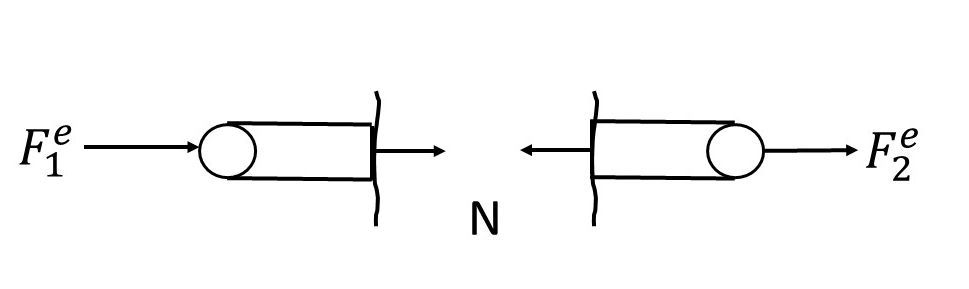
Equilibrium of the element given in the figure, id est the sum of the forces applied on each node of the element is equal to zero (F^e_1 + F^e_2 = 0).
As we can see in the figure above we apply two forces at the beginning and the end of our bar e so that our system is in equilibrium. If we look now at the balance of powers in matrix notation (tensor notation), we get
The matrix \underline{\underline{K}}^e is called the element stiffness matrix is symmetric and positive semi-definite. The vector \underline{d}^e is called the element displacement matrix and \underline{F}^e the element internal force matrix. The stiffness matrix establishes the correlation between nodal displacements and nodal forces.
Keep in mind that the matrix \underline{\underline{K}}^e is always singular meaning in the sense of mathematics that the matrix is not invertible. We can also see that in our matrix if we add the rows together (+1 - 1 = 0). The mechanical interpretation for this phenomenon is that our bar is able to undergo rigid body motions. Positive semi-definite (Definite quadratic form) follows from the non-negativity of the deformation energy of our bar for arbitrary nodal displacements \underline{d}^e (We have always mechanical input in our system! No matter if it is tension or compression!)
4.2 Correlation between local and global quantities
We just looked at element-wise (local) quantities, for instance the element internal force matrix \underline{F}^e and the element displacement vector \underline{d}^e. In an assembled system we can describe local and global quantities with so called gather matrices \underline{\underline{L}}^e which are Boolean matrices because they only consist of zeros and ones.
On the one hand we can determine the nodal displacements correlated to our element e from the global displacement vector \underline{d}^e
On the other hand we have the external forces F_i. The sum of all F_i have to be equal to the components of the element internal force matrix. In order to scatter the components of the element internal force matrix into the global force matrix \underline{F} we have
Considering (5) and (7) we get the following expression
The vector \underline{d} is independent of the element index treating it like a factor and put it in front of our sum
The matrix \underline{\underline{K}} is called global stiffness matrix. This matrix is compared to \underline{\underline{K}}^e also symmetric and positive semi-definite. The linear system of equations in (10) is not solvable since we are missing something very important: Boundary conditions!
We will come back to the boundary conditions a bit later but now let us look at an example which gives you a deeper understanding of gather matrices ![]()
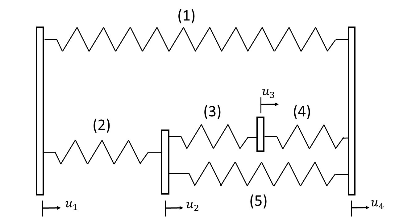
Spring System without boundaries
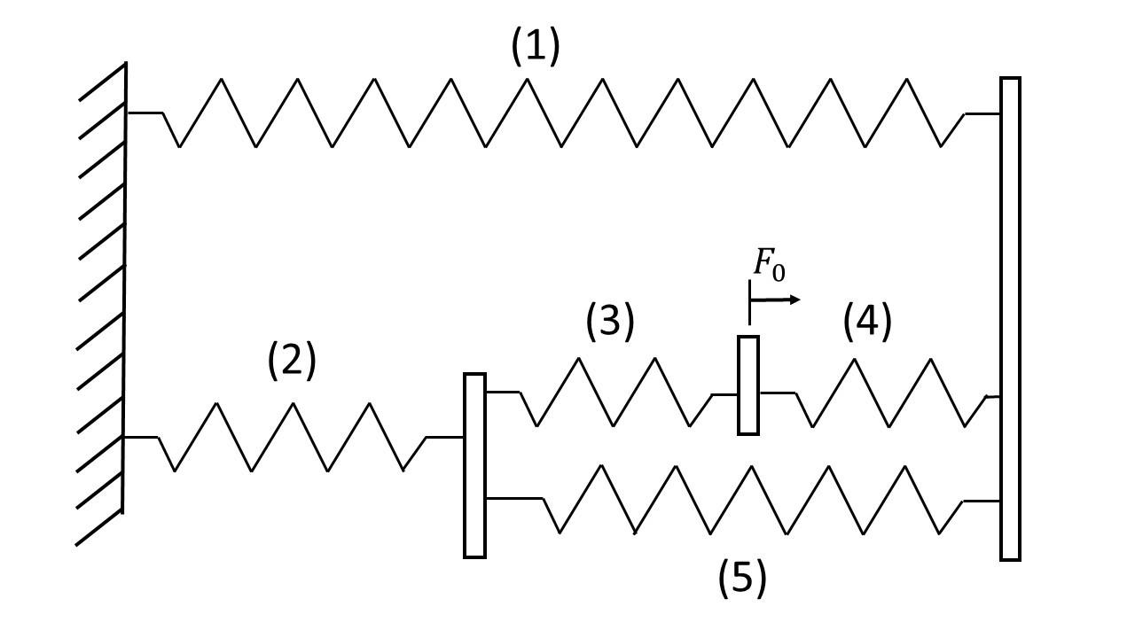
Spring System with boundaries
In the system given above we have n_{vx}=4 nodes and n_e=5 elements. The gather matrices chose the relevant displacements from the global displacement vector \underline{d} = \begin{bmatrix} u_1 , u_2 , u_3 , u_4 \end{bmatrix}^\intercal . The dimension depends of the gather matrix depends on the number of nodes of the element and the number of DOFs (Degrees of freedom). In our example we have a 2 x 4 matrix which choses the two relevant displacements from the possible four displacements.
Gather matrices have the following dimensions
For the given system we have the following combination of gather matrices
To get the stiffness of an element we look at element nr.5 of our system.
Our gather matrix for this element is
The force vector applied at the element is a combination of the applied forces at the element nodes
where F^{(5)}_2 defines the contribution of the fifth element to the nodal force F_2. If we now create the transposed of the gather matrix we can identify the contribution of the fifth bar element to the global force vector
The element stiffness matrix of the fifth element is defined as
If we now calculate \underline{\underline{L}}^{(5)^\intercal} \underline{\underline{K}}^{(5)} \underline{\underline{L}}^{(5)} we get the contribution of the fifth element to the global stiffness matrix as shown below
If have a bit of practice, you can easily write down the solution of \underline{\underline{L}}^{(5)^\intercal} \underline{\underline{K}}^{(5)} \underline{\underline{L}}^{(5)} by just looking at the system (if it is simple).
4.3 Boundary conditions
As mentioned previously, our linear system of equations (10) is underconstrained. The reason is that we can still undergo the system with a rigid body motion. If we displace our system by a constant value u_0 it hast absolutely no impact on the global force vector. At this point we need boundary conditions of the type: Dirichlet-Boundary.
In order to consider Dirichlet-Boundaries in the discrete mechanical system, we partition the displacement vector \underline{d} into free nodel displacements \underline{d}_f (unknown) and prescribed nodal displacements \underline{d}_e (e:“essential”). For this purpose we define the new gather matrices \underline{\underline{L}}_E and \underline{\underline{L}}_F. We then have
where \underline{d}_F define the unknown displacements.
The matrix \underline{\underline{L}}_E holds n_{vx} (DOFs) rows and n_D columns, where n_D is the number of prescribed displacements from the Dirichlet-Boundaries. The matrix \underline{\underline{L}}_F has an equal number of rows but n_F = n_{vx} - n_D columns. For this gather matrices the following connectedness holds
Furthermore the vector of exterior forces includes ,besides prescribed forces, also unknown reaction forces. Those are exactly at the points where the Dirichlet-Boundaries is. The force vector can be partitioned in the following manner
where \underline{r} \in \mathbb{R}^{n_D} is equal to the unknown reaction forces.
4.4 Derivation of the reduced system of equations
(19) and (21) can be plugged into the system of equation (10). Considering (20) we can write
with the following short form
result to the following two linear systems
The unknowns in these two systems are \underline{r} and \underline{d}_F where the reaction force vector \underline{r} is linearly dependent of \underline{d}_F. The free nodal displacement vector \underline{d}_F can be determined directly from the second equation IF we have enough boundaries of type Dirichlet defined. We can do this because the Matrix \underline{\underline{K}}_{FF} is symmetric and positive definite, especially regular (det \neq 0). We call the matrix \underline{\underline{K}}_{FF} reduced stiffness matrix and the corresponding system reduced system. We get the solution with the following two steps:
• Calculation of \underline{d}_F = \underline{\underline{K}}^{-1}_{FF} (\underline{F}_F - \underline{\underline{K}}_{FE} \underline{d}_E) In practice we never calculate the inverse of \underline{\underline{K}}_{FF} but solve the corresponding system of equations with a direct or iterative method which we will learn at the end of this course
• Plug in the equation for the unknown reaction forces
Displacement- and Force boundaries can never be prescribed at the same time for the same node. Otherwise our problem would be overconstrained. A common mistake SimScale users encounter when prescribing two boundaries for the same point/face. We all did it once, admit it. ![]()
The last step is the application of what we learned. Therefore we will do one example and are already finished with this chapter ![]()
Three-bar problem
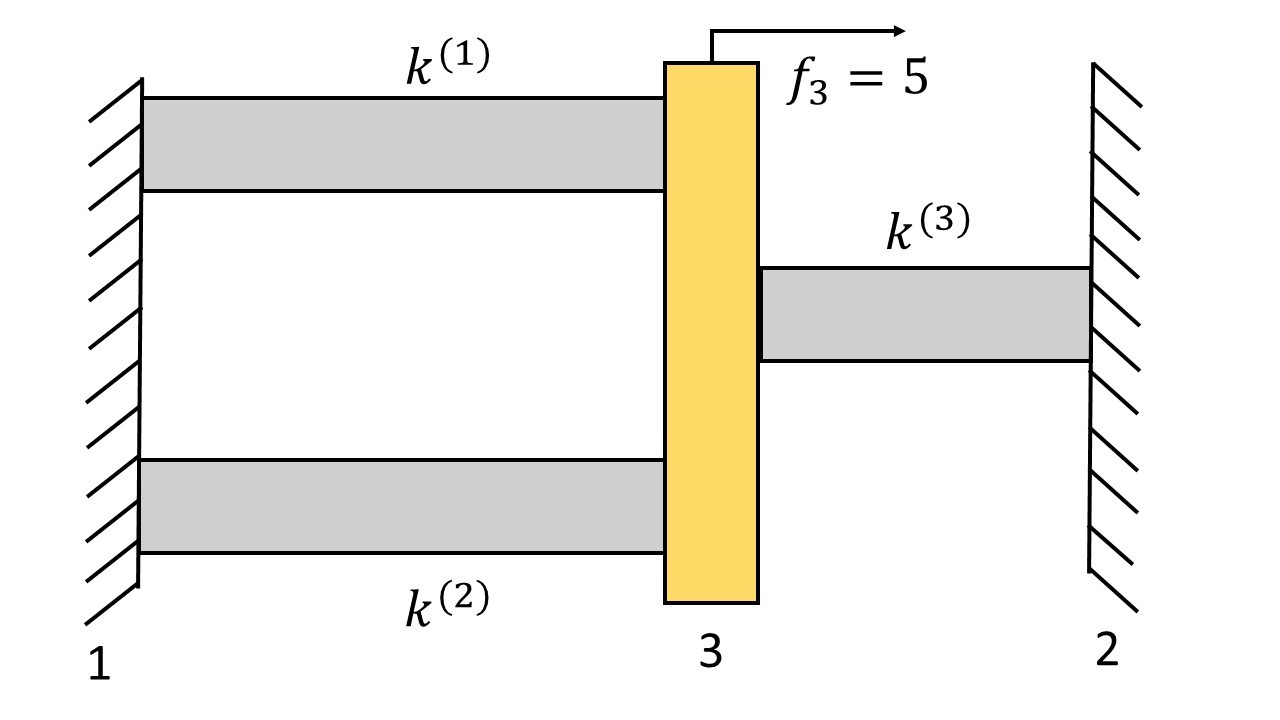
The element stiffness matrices are
The global stiffness matrix is (can be easily obtained by direct assembly)
The displacement and force matrices are
The global system is given by
We now partition the matrix after two rows and columns because the first two displacements are prescribed
or
The reduced system of equations is given by
which finally gives us the displacement u_3 as
Sources:
• Introduction to the Finite Element Method - Niels Ottosen & Hans Petersson
• A First Course in Finite Elements by Jacob Fish and Ted Belytschko
• Lectures of KIT Karlsruhe (Script: Einführung in die Finite Elemente Methode Sommersemester 2014)
This was the fourth part for FEM fundamentals. The following chapter will provide be about the strong and weak form of the differential equations in FEM.
If you find any mistakes or have wishes for the next chapters please let me know.
Scientia potentia est!
First chapter: The Finite Element Method - Fundamentals - Introduction [1]
Second chapter: The Finite Element Method - Fundamentals - Physical Problems [2]
Third chapter: The Finite Element Method - Fundamentals - Matrix Algebra [3]