Hello guys and welcome to my first post for FEM fundamentals.
As an introduction watch the following video of the well known Gilbert Strang

FEM - A Beginner’s Guide
 - A Beginner's Guide")
History and background of the Finite-Element-Method
History & Facts
• The term Finite Element was introduced 1960 by Ray William Clough (Berkeley). In the early 60s this method has been used by several engineers for stress analysis, fluid transport, heat transport and other subjects
• The first Finite-Element-Method book has been published by Zienkiewicz and Chung
• In the late 60s and 70s the field of FEM application expanded and became a leading numerical approximation in a broad field of engineering problems
• Most commercial codes like ANSYS, ABAQUS, Adina and several others have their origin in the 1970s
• The US spend more than $1 billion annually on software and computer time
• A web search (2006) for ‘finite element’ using Google yielded over 14 million pages
• Mackerle lists 578 finite element books published between 1967 and 2005
• For linear systems, nodal values are obtained by solving large systems of linear algebraic equations (103 to 106 is common, and in special applications 109)
• FEM systems at Mercedes in the early beginnings have been solved by punchcards
Motivation
We use the finite element method for several reasons. Analytical models are limited in their application. This is the case if we have:
• complex geometries
• complex loadings (point of force application,…)
• material laws, for instance
   - Anisotropic material law (fibre-reinforced plastic or crystalline material)
   - inhomogeneous material properties (Young’s modulus…)
Numerical Methods
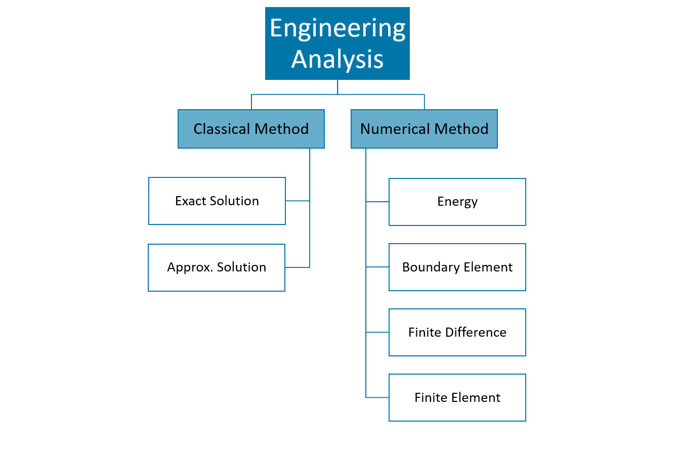
Approach of the Finite-Element-Method
Physical phenomena in general can be described with differential equations. Differential equations describe nature. Those partial differential equations (PDE) are solved in an approximate manner by the finite element method (FEM).
The following five steps are essential to know in order to understand what the approach of the FEM is:
First step (Preprocessing):
• Create geometry
• Define material properties
• Choose initial and boundary conditions
• Define (if necessary) side conditions like contact definitions
• Discretization of the geometry → MESH
Second step:
Element formulation → development of equations for elements
Set up the partial differential equation in its weak form
Third step:
Assembly: Set up global problem → obtaining equations for the entire system from the equations for one element
Fourth step:
Solving the equations (solve system of linear equations)
Fifth step:
Postprocessing: determining quantities of interest, such as stresses and strains and obtaining visualizations of the response
Hint: The solver may produce super cool, colourful results which may look convincing but may be irrelevant. So try to compare your solution with analytical results (if available).
DIVIDE AND CONQUER!
A characteristic feature of the finite element method is that instead of seeking the approximation over the entire region, the region is divided into smaller parts, so called finite elements and the approximation is then carried out over each element. The collection of all small parts is called the finite element mesh.
When the type of approximation has been chosen (is to be applied over each element), the corresponding behaviour of each element can then be determined. Having determined the behaviour of all single elements, the elements can then be patched together, which hopefully enables us to get an approximate solution of the entire body.
In this course we are only concerned with boundary value problems (BVP), i.e. differential equations where some information is known a priori. We can even solve initial value problems like wave propagation and transient heat conduction with this method.
As we mentioned before we need to approximate over our elements in order to determine the behaviour. This approximation is usually a polynomial and is, in fact, some interpolation over the element. This means we know some values at certain points within the element but not at every point. These ‘certain points’ are called nodal points and are often located at the boundary of the element. The accuracy with which the variable changes is expressed by the approximation, which can be linear, quadratic, cubic et cetera.
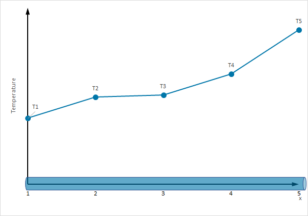
In order to get a better understanding of approximation techniques, we will look at a one-dimensional bar. Consider the true temperature distribution T(x) along the bar in the picture below.
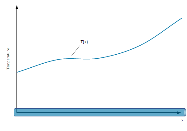
The nodal points we chose do not need to be equally spaced (as we see in later chapters).
We divide our bar into four elements over which the temperature is assumed to vary in a linear manner between each nodal point!
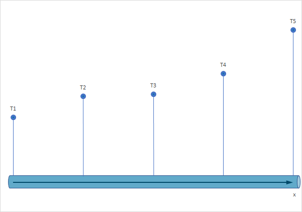
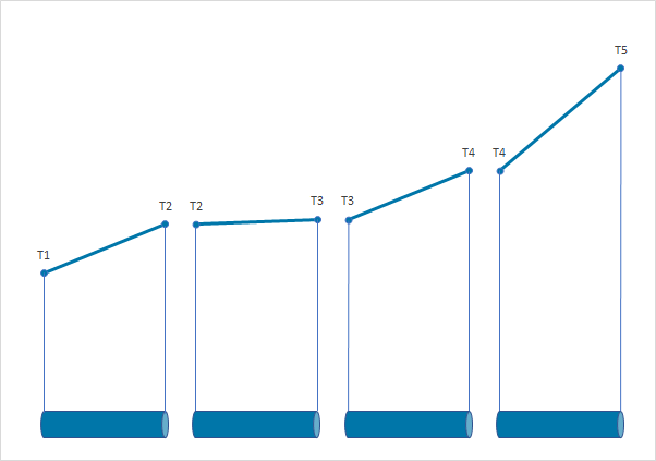
Well we see linear approximation is quite good but we can do it better! If we chose a quadratic approximation the temperature distribution along the bar is way more smooth. Nevertheless, we see that irrespective of the polynomial degree the distribution over the fin is known once we know the values at the nodal points, simple as that. If we just have one bar we would have an infinite amount of unknowns (DEGREES OF FREEDOM (DOF)). But in this case we have a problem with a finite number of unknowns.
A system with a finite number of unknowns is called a discrete system.
A system with an infinite number of unknowns is called a continuous system.
In our case we would have a system consisting of five equations which can be solved by hand but in general we have thousands and thousands of unknowns. Have fun solving this by hand. Luckily we have efficient computers solving such kind of problems for us which makes life way easier ![]() .
.
Sources:
• Introduction to the Finite Element Method – Niels Ottosen & Hans Petersson
• A First Course in Finite Elements by Jacob Fish and Ted Belytschko
• Partial differential equation - Wikipedia
• Lectures of KIT Karlsruhe (Script: Einführung in die Finite Elemente Methode Sommersemester 2014)
This was the first post for FEM fundamentals. The next chapter will be about physical problems like elastostatics and heat conduction which will be short. The following chapter will provide a review of basic matrix algebra.
If you find any mistakes or have wishes for the next chapters please let me know.
Chapter 2: The Finite Element Method - Fundamentals - Physical Problems [2]
Show your appreciation with a like or buy me a cookie. ![]()
![]()


 Thank you very much for your appreciation!