Link to part 1 of the tutorial:
Step-by-Step Tutorial Session 2 - Full Car Aerodynamics (Part 1)
Introduction
Welcome to the second part of the step-by-step tutorial for the simulation of a Formula SAE full car. In this part of the tutorial we will show you the final steps for the simulation setup and we will go over the post processing of the results. Like last session, we will also go through some of the results and what they mean.
Simulation Setup (Part 2)
Advanced Concepts
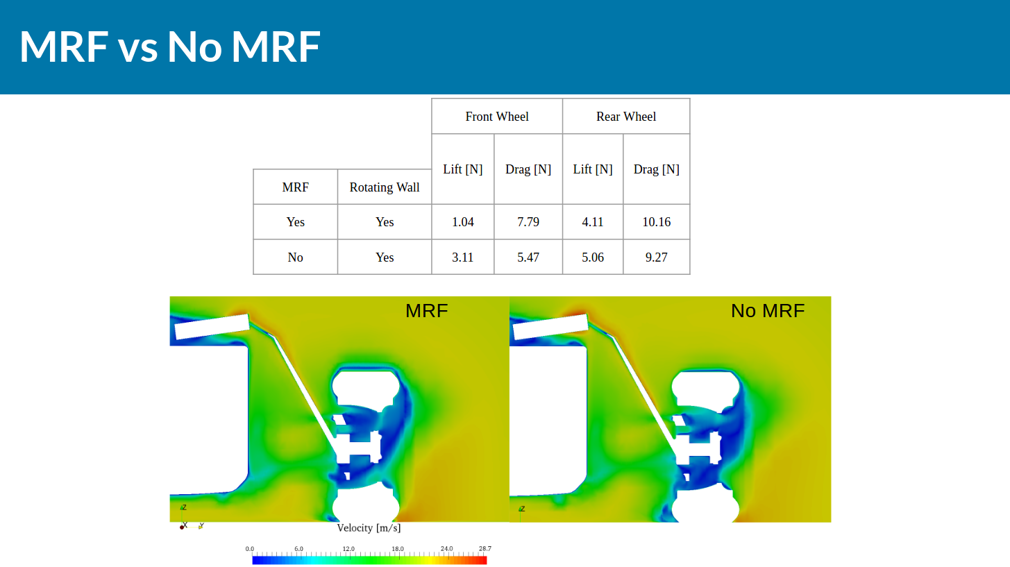
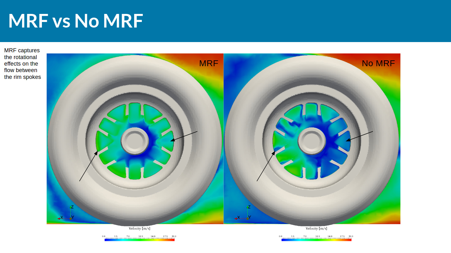
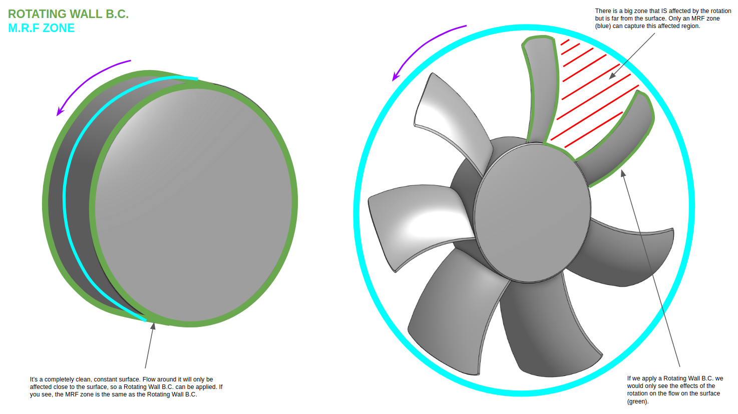
Rotating Wall Boundary Conditions vs Multi Reference Frame (MRF)
You have just added a Rotating Wall Boundary Condition in part 1, and now you will add the MRF zones. The difference between a rotating wall boundary condition and the MRF zone comes down mainly to the geometry. Here’s how it works: the rotating wall allows us to correctly simulate the effects of the rotational solid on the fluid close to the surface of the solid. This works well when you have a simple geometry like a cylinder (essentially these tires). We could apply an MRF zone to the tires too, but this would be computationally more expensive and not necessary because the tire is only affecting the flow close to its surface. On the other hand, the spokes of the wheel rim not only affect the flow close to their surface but around a much bigger zone, and this zone is the one we define as an MRF zone. Refer to the following image for a visual explanation.
Rotating Zones
Now we will finally create the MRF zones for the wheel rims.
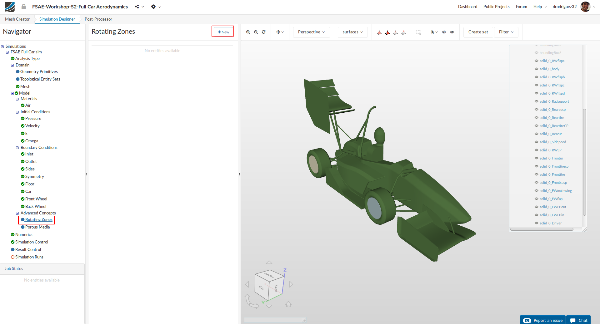
Go to Advanced Concepts and click on Rotating Zones in the navigator on the left. Then click on New to setup a new rotating zone.
MRF Front
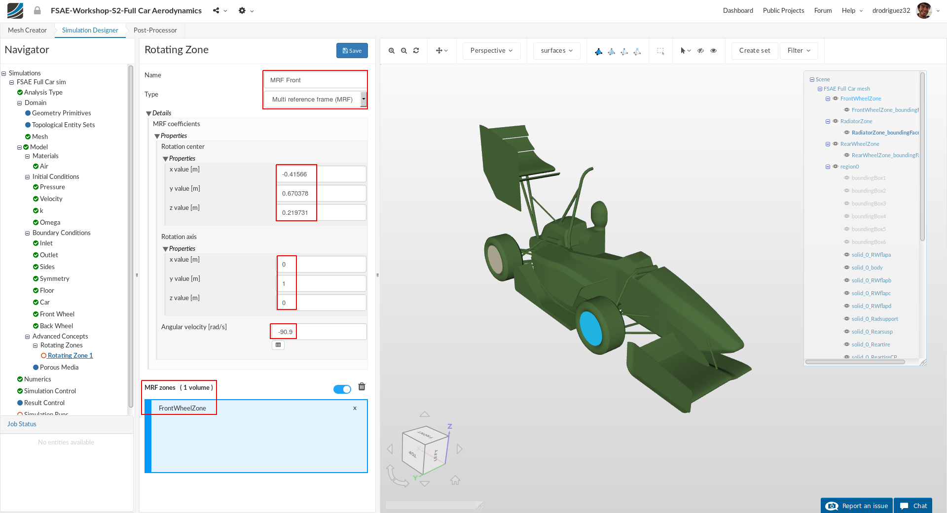
Now rename it to MRF Front
Then change:
-
Origin x value [m], y value [m] and z value [m] value to -0.41566, 0.670378 and 0.219731 respectively.
-
Axis of rotation y value [m] to 1
-
Angular velocity [rad/s] to -90.9
-
Then select FrontWheelZone. You should see it in the blue highlighted box under MRF zones and highlighted in blue in the viewer.
-
Make sure your settings match the picture and then click Save to register your changes.
MRF Rear
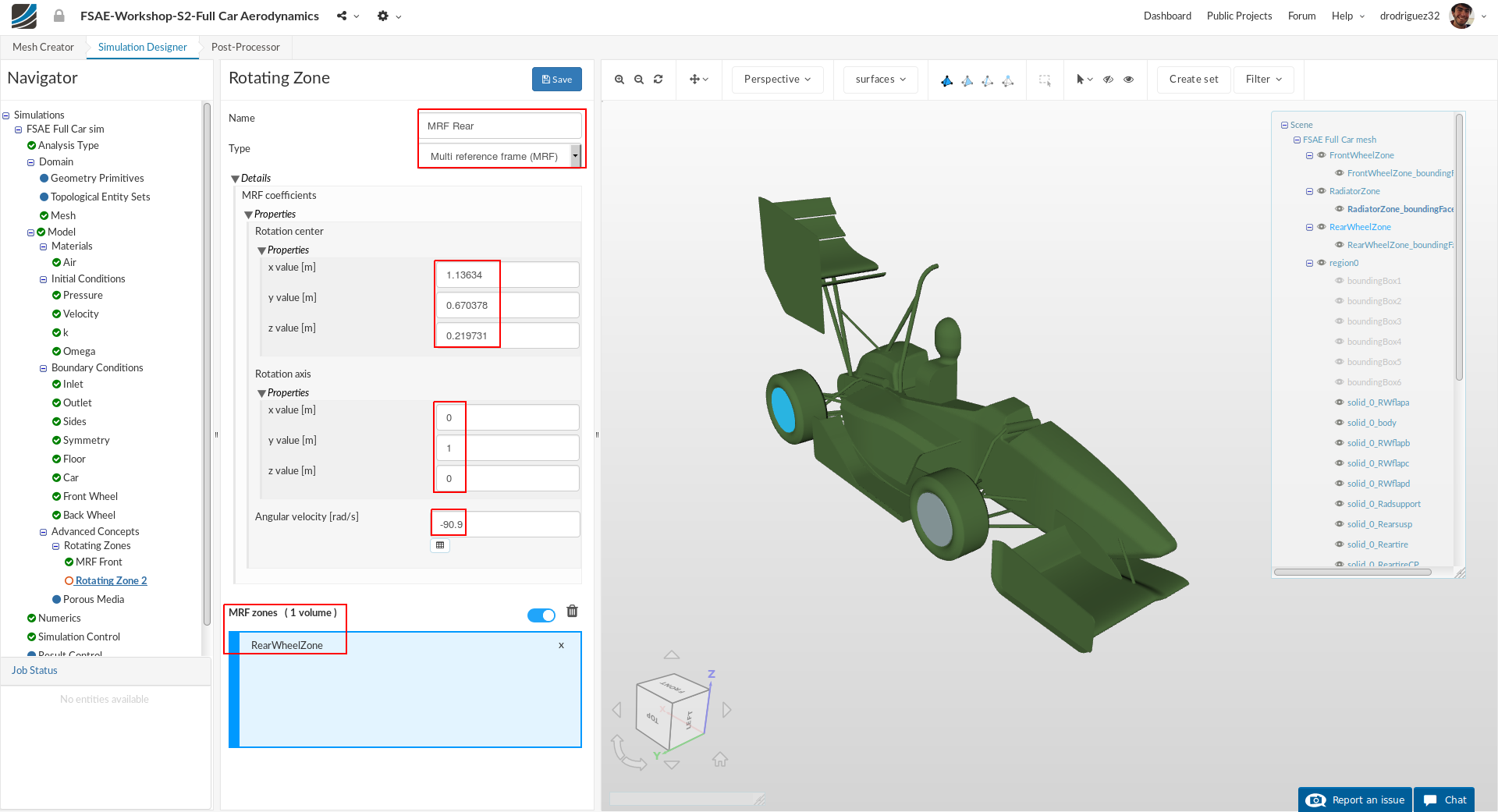
Similarly, perform the same procedure and create a new Rotating Zone. Rename it to MRF Rear. Then change:
-
Rotation center x value [m], y value [m] and z value [m] value to 1.13634, 0.670378 and 0.219731 respectively.
a. Notice that the values for the y axis and z axis are the same as for the front wheel -
Rotation axis y value [m] to 1.
-
Angular velocity [rad/s] to -90.9
-
Then select RearWheelZone. You should see it in the blue highlighted box under MRF zones and highlighted in blue in the viewer.
-
Click Save to register your changes.
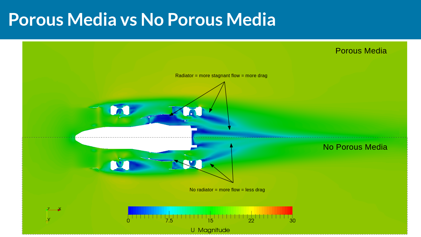
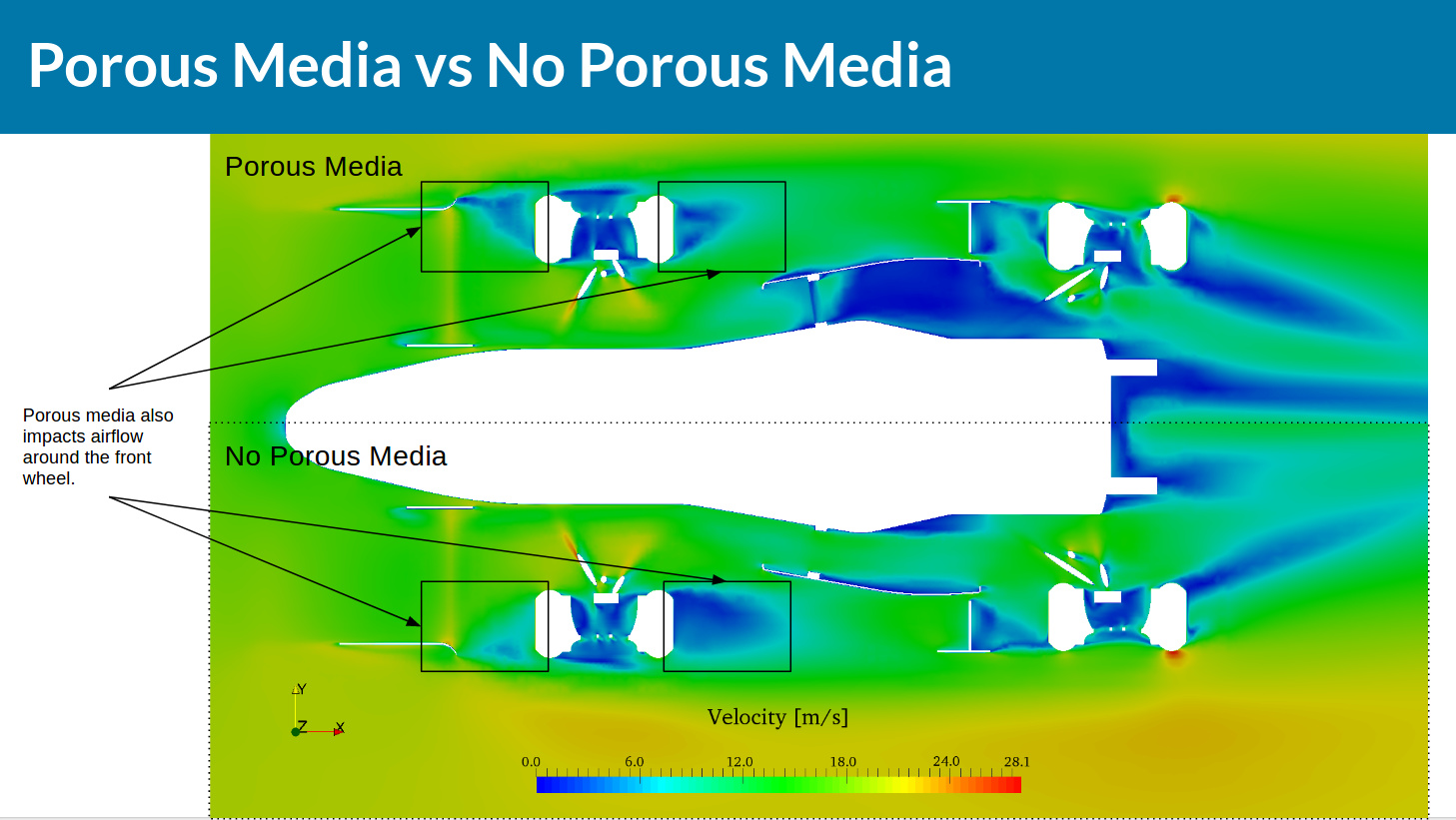
Porous Media
In this section we will define the radiator via porous media. In the real world there are many things that are very complex for a simulation to be viable. A perfect example of this is turbulence, and as we already explained, instead of having an ridiculously fine mesh, we apply some mathematical models that predict the turbulence with enough accuracy to make engineering decisions. Porous objects present a similar challenge for simulations: imagine how refined a mesh would have to be in order to capture all the details (tiny holes and structures) of a sponge, an air filter, or in this case a radiator. So to solve this, we use the porous media approach. This approach adds some terms to the equations that are being solved for the cells in that zone so that the behavior of the porous solid can be predicted correctly. These equations take into account the porosity and the mean particle diameter to observe the effects on the flow and the inertial effects when you have high velocity flow. To read more about this go to Porous Media in the SimScale documentation.
As you saw in the presentation, when you have experimental results for the radiator you get a curve of pressure drop vs fluid flow. This curve can be closely approximated using a second order polynomial such that:
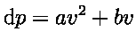
When you have obtained the coefficients ‘a’ and ‘b’, you proceed to these next equations to calculate the vectors for ‘d’ (Darcy coefficient) and ‘f’ (Forchheimer coefficient):
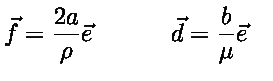
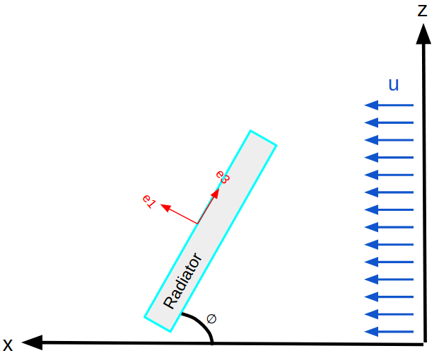
In these equations, vector ‘e’ refers to a vector that should be aligned with the local flow direction. This simply means that it should be orthogonal to the radiator face and pointing in the flow direction as shown by ‘e1’ in this image:
When you have all the vectors defined (don’t worry you don’t have to calculate them this time) you can move onto the platform and setup your porous media.
Radiator
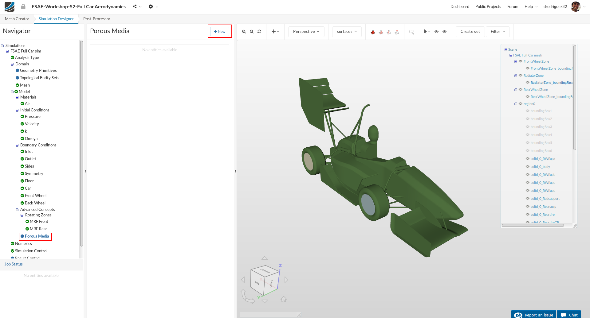
Expand the Advanced Concepts tree item and proceed to Porous Media. Click +New to create a new porous media definition.
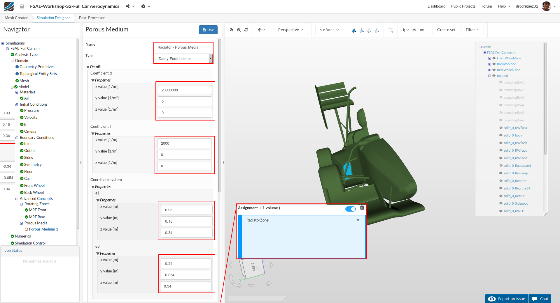
After creating a new porous media definition, you will be automatically directed to the its properties panel. Now that you know how porous media works you can apply it to your own designs. For the sake of simplicity, we have made an approximation of the coefficients of this radiator to make it simpler and more straight forward. The vector is the correct calculated normal for the local flow direction. Change:
-
Name to Radiator - Porous Media (optional) and set the Type to Darcy-Forchheimer
a. This Darcy-Forchheimer is the model that will be used. The Darcy part states that the flow through the porous medium is proportional to the pressure drop. The Forchhiemer part is a nonlinear term for flows with high reynolds numbers that takes into account the inertial effects. -
Coefficient d x, y and z values to 20,000,000, 0, and 0 respectively.
a. This is the Darcy coefficient, or the linear part of the model. -
Coefficient f x, y and z values to 2000, 0, and 0 respectively.
a. This is the Forchheimer coefficient… -
Coordinate system e1 x, y and z values to 0.93, 0.15 and 0.34 respectively.
a. This is the vector that tells the model the local flow direction. -
Coordinate system e3 x, y and z values to -0.34, -0.054 and 0.94 respectively.
a. This is a vector that is orthogonal to e1. -
Scroll down and select RadiatorZone from the navigator on the right. Make sure it appears in the blue box under Assignment.
-
Click Save to register your changes.
Numerics
After defining all the boundary conditions, we will proceed to set up the numerics for our simulation.
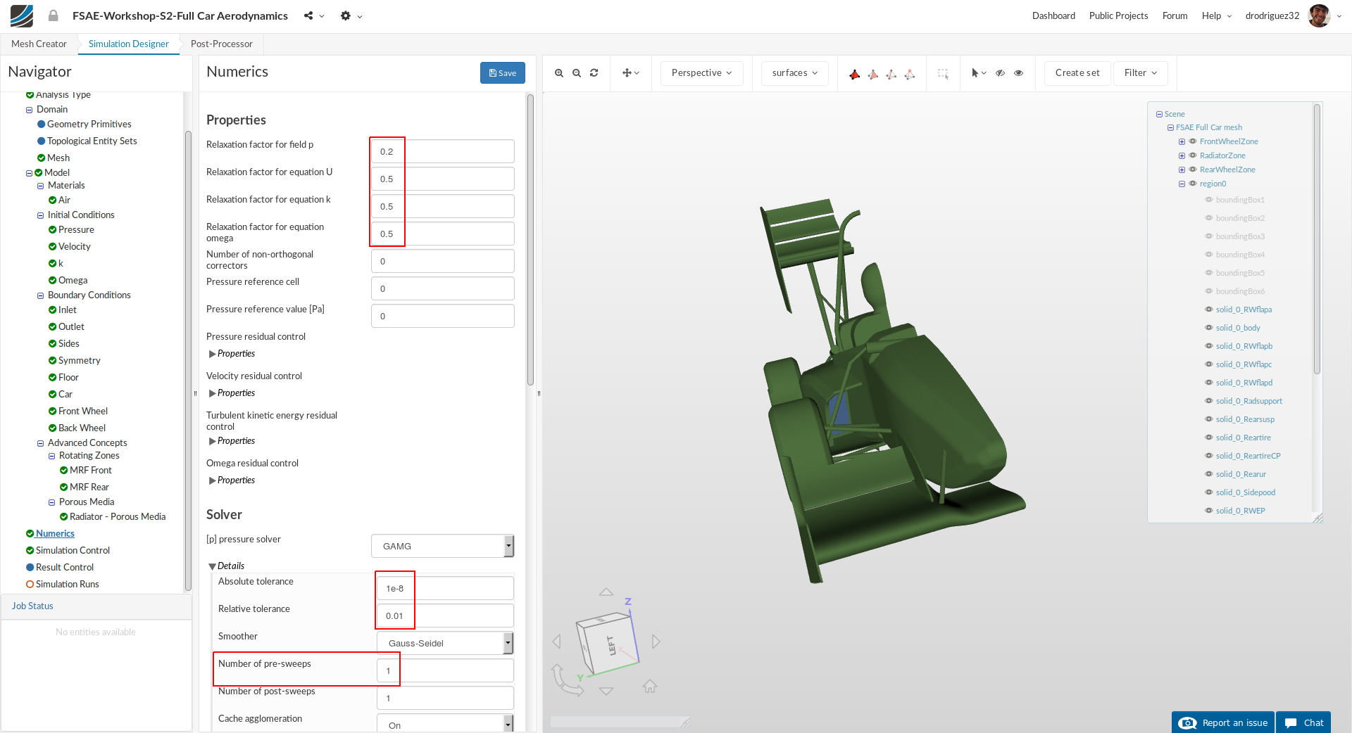
Go to Numerics and change:
-
Relaxation factor for field p, Relaxation factor for equation U, Relaxation factor for equation k and Relaxation factor for equation omega to 0.2, 0.5, 0.5 and 0.5 respectively.
-
Furthermore, under [p] pressure solver, change Absolute tolerance, Relative tolerance and Number of pre-sweeps to 1e-8, 0.01 and 1 respectively.
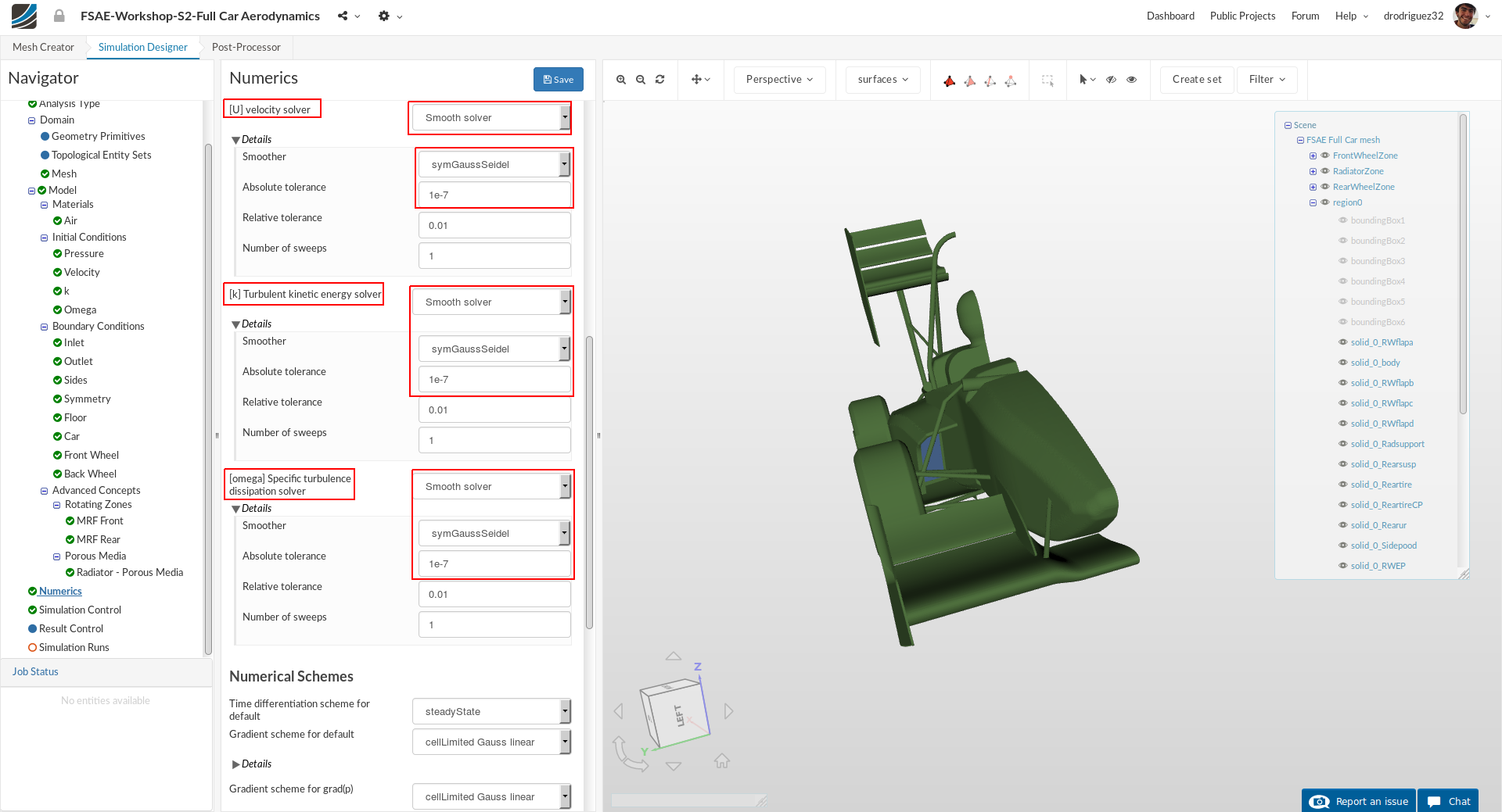
Scroll down until [U] velocity solver and change:
-
[U] velocity solver to Smooth solver, Smoother to symGaussSeidel and Absolute tolerance to 1e-7. Do the same for [k] Turbulent kinetic energy solver and [omega] Specific turbulence dissipation solver.
-
Change both Gradient scheme for default and Gradient scheme for grad p to cellLimited Gauss linear
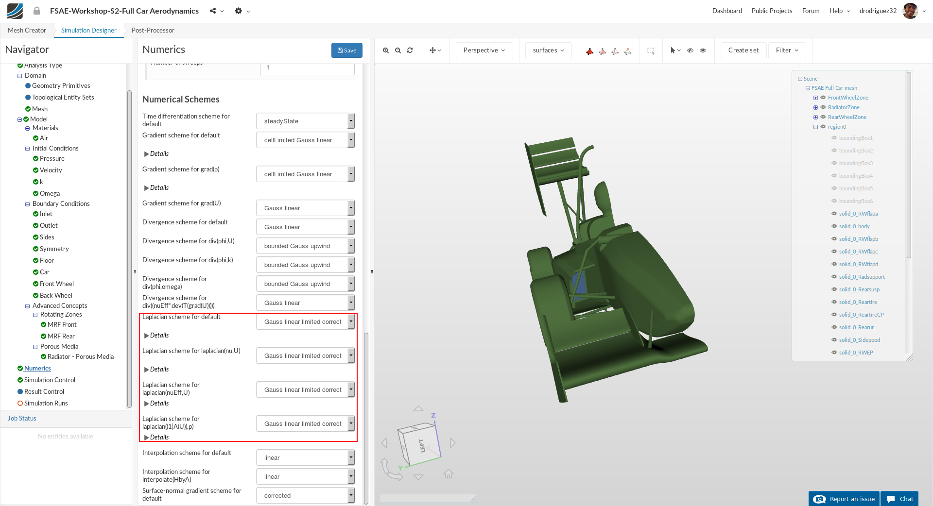
Scroll down to the end and change:
-
Laplacian scheme for default, Laplacian scheme for laplacian(nu,U), Laplacian scheme for laplacian(nuEff,U) and Laplacian scheme for laplacian((1|A(U)),p) to Gauss linear limited corrected
-
Click Save to register all of your changes.
Simulation Control
Next we will define our simulation interval and steps that needs to be recorded.
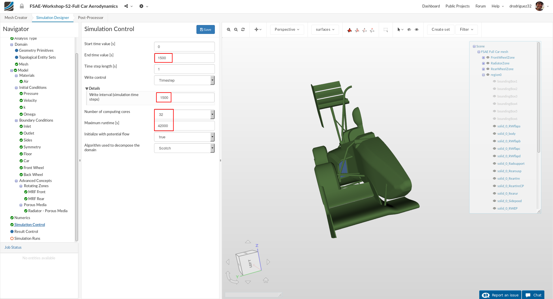
Go to Simulation Control and change End time value [s] to 1500.
Expand Details under Write control and change Write interval (simulation time steps) to 1500.
Next change Number of computing cores and Maximum runtime [s] to 32 and 42000 respectively.
Click Save to register your changes.
Result Control
As our last step before running the simulation, we will create result control items in order to get graphical data sets of interest.
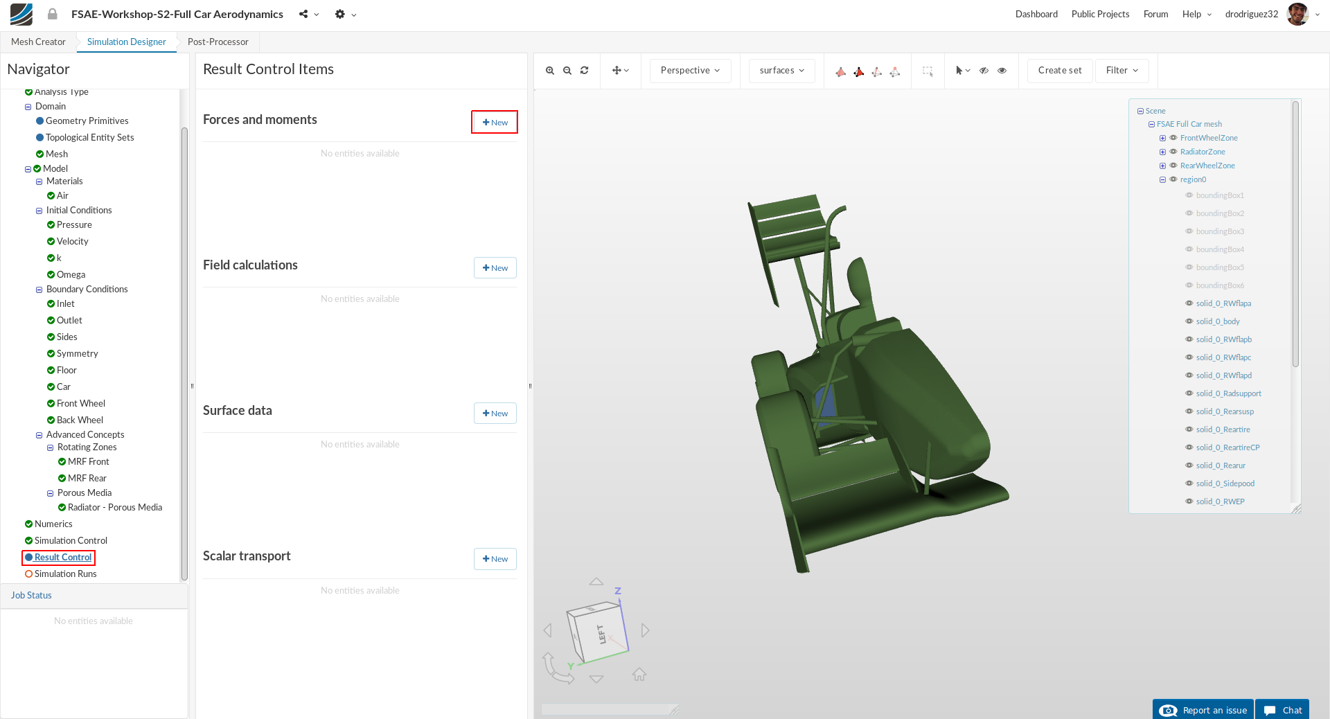
Firstly, we will create the result control item for the forces and moments. Go to Result Control and click New next to Forces and Moments.
A new force and moment result control item will be created.
Front Wing
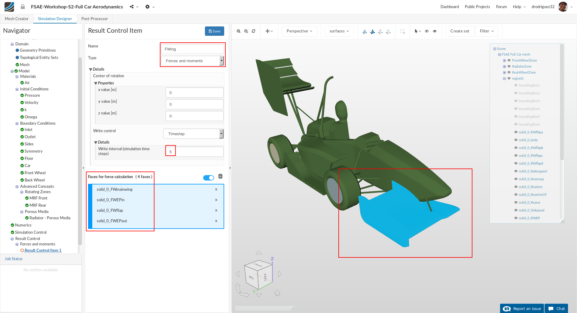
Rename it to FWing (optional).
Then change Write interval (simulation time steps) 5.
Select solid_0_FWmainwing, solid_0_FWEPin, solid_0_FWEPout and solid_0_FWflap. You should see them under Faces for force calculation.
Click Save to register your changes.
Rear Wing
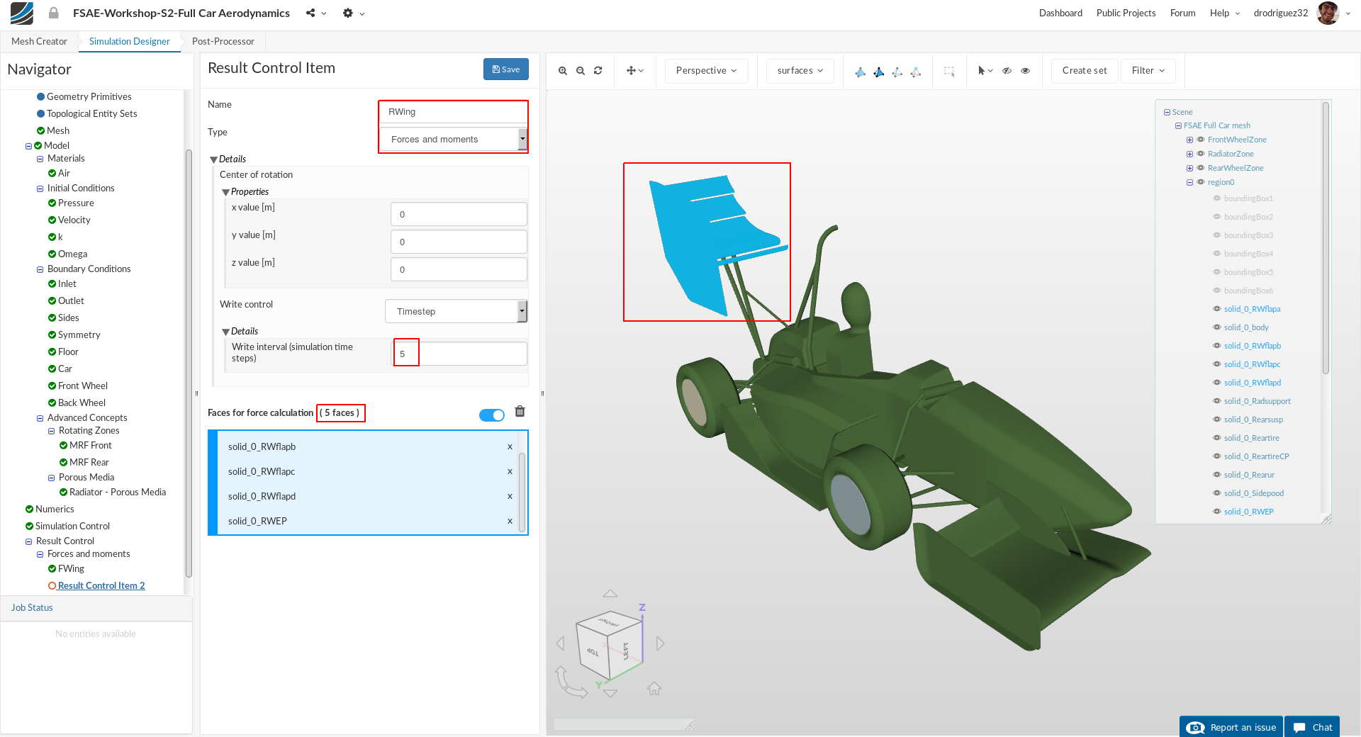
Create another force and moment result control item and rename it to RWing (optional).
Then change Write interval (simulation time steps) 5.
Select solid_0_RWEP, solid_0_RWflapa, solid_0_RWflapb, solid_0_RWflapc and solid_0_RWflapd. You should see them under Faces for force calculation.
Click Save to register your changes.
Diffuser
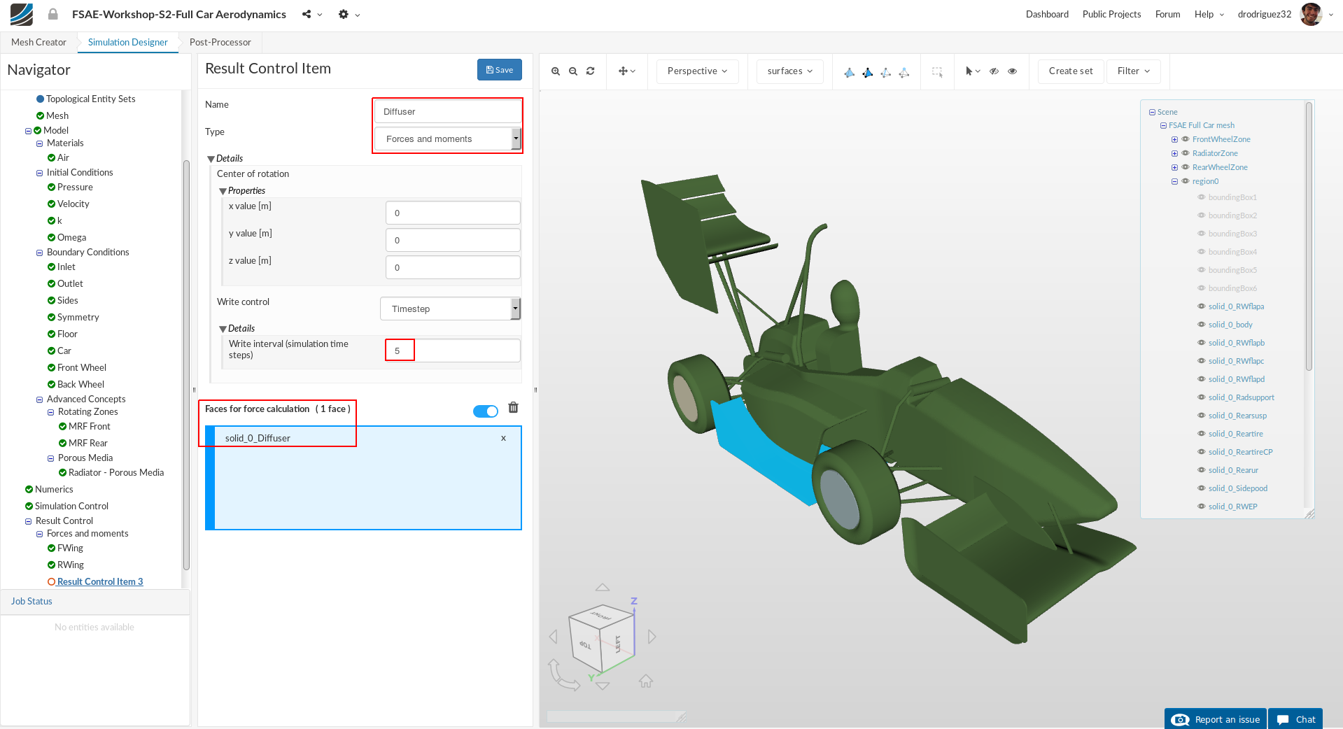
Follow the same procedure to create force and moment result control item for the diffuser. Rename it to Diffuser (optional).
Then change Write interval (simulation time steps) 5.
Select solid_0_Diffuser.
Click Save to register your changes.
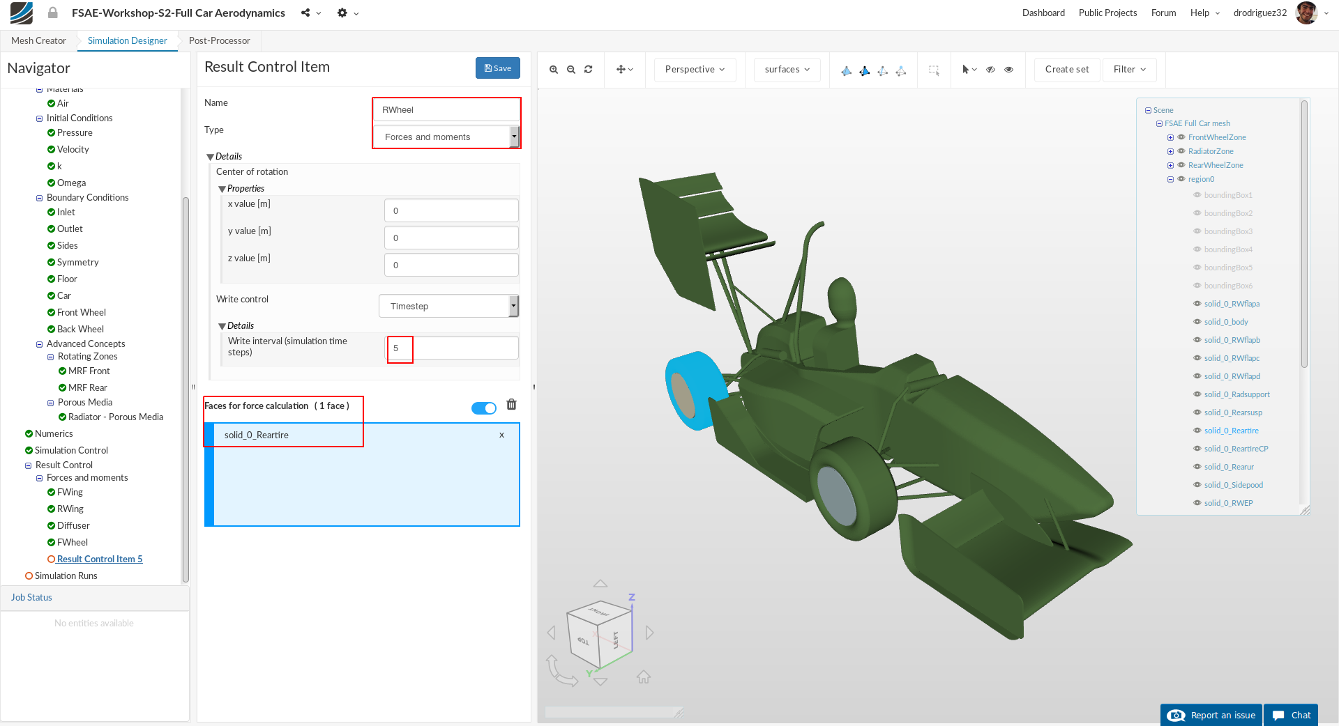
Front Wheel
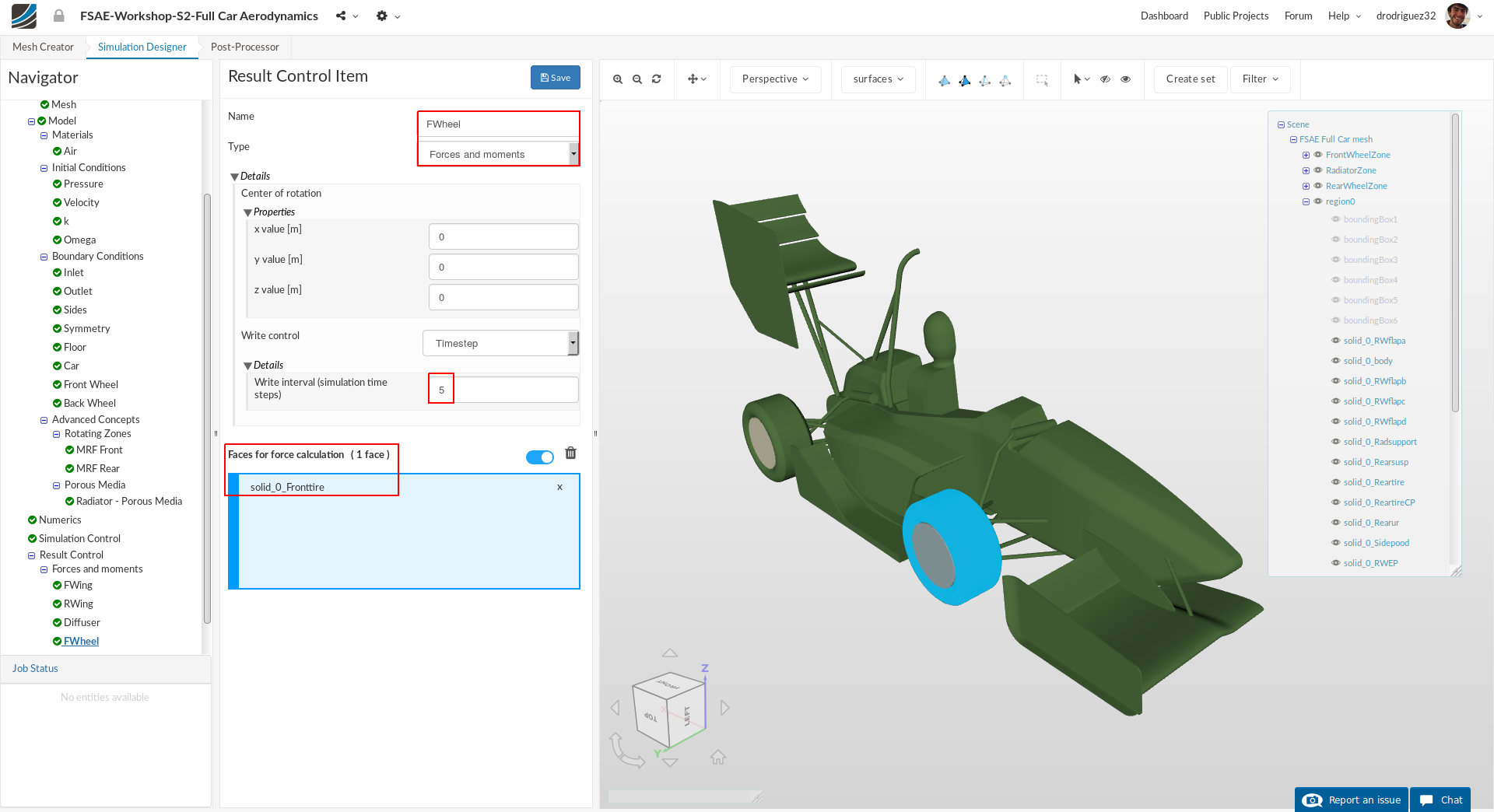
Follow the same procedure to create force and moment result control item for the front wheel and rename it to FWheel (optional).
Then change Write interval (simulation time steps) 5.
Select solid_0_Fronttire.
Click Save to register your changes.
Rear Wheel
Do the same for rear wheel, rename it to RWheel (optional).
Then change Write interval (simulation time steps) 5.
Select solid_0_Reartire.
Click Save to register your changes.
Body
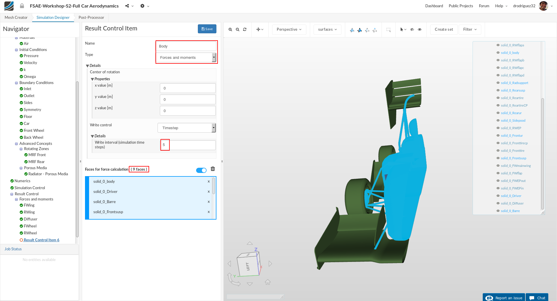
Similarly, for the whole body repeat the procedure and this time rename it to Body (optional).
Then change Write interval (simulation time steps) 5.
Select solid_0_body, solid_0_Frontsusp, solid_0_Rearsusp, solid_0_Barre, solid_0_Sidepood, solid_0_Frontur, solid_0_Radsupport, solid_0_Rearur and solid_0_Driver.
Make sure you have the 9 surfaces selected. They should be blue in the viewer, the names should appear in the highlighted area under Faces for force calculation and they should also be highlighted in the navigator on the right. Click Save to register your changes.
Simulation Run
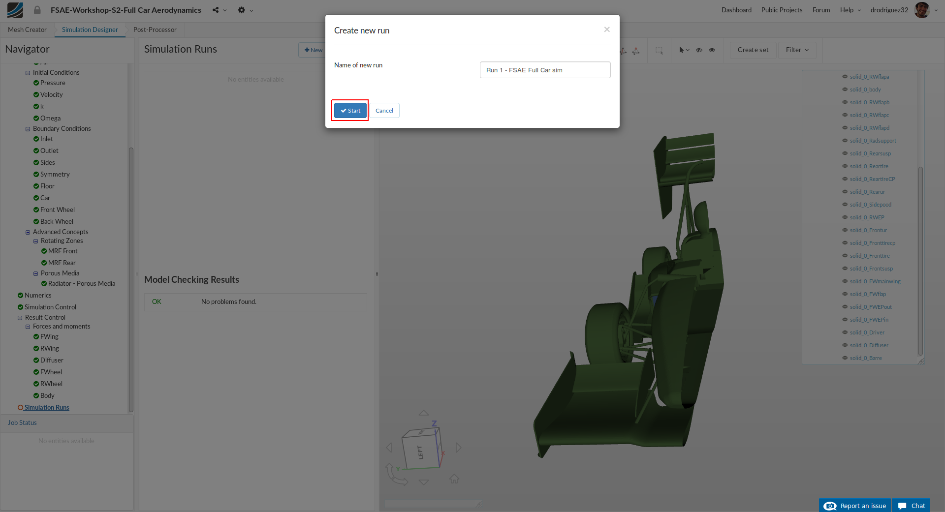
Once all the above steps are defined, we will proceed to create our first simulation run. Go to Simulation Runs and click on New and then Create in order to create a new run.
After the run is created, click Start to start the created run. The simulation run can take up to ~200 minutes (~3.3 hrs.)
Post-processing on SimScale
Once your simulation is completed, proceed to Post-Processor tab in order to post-process your results.
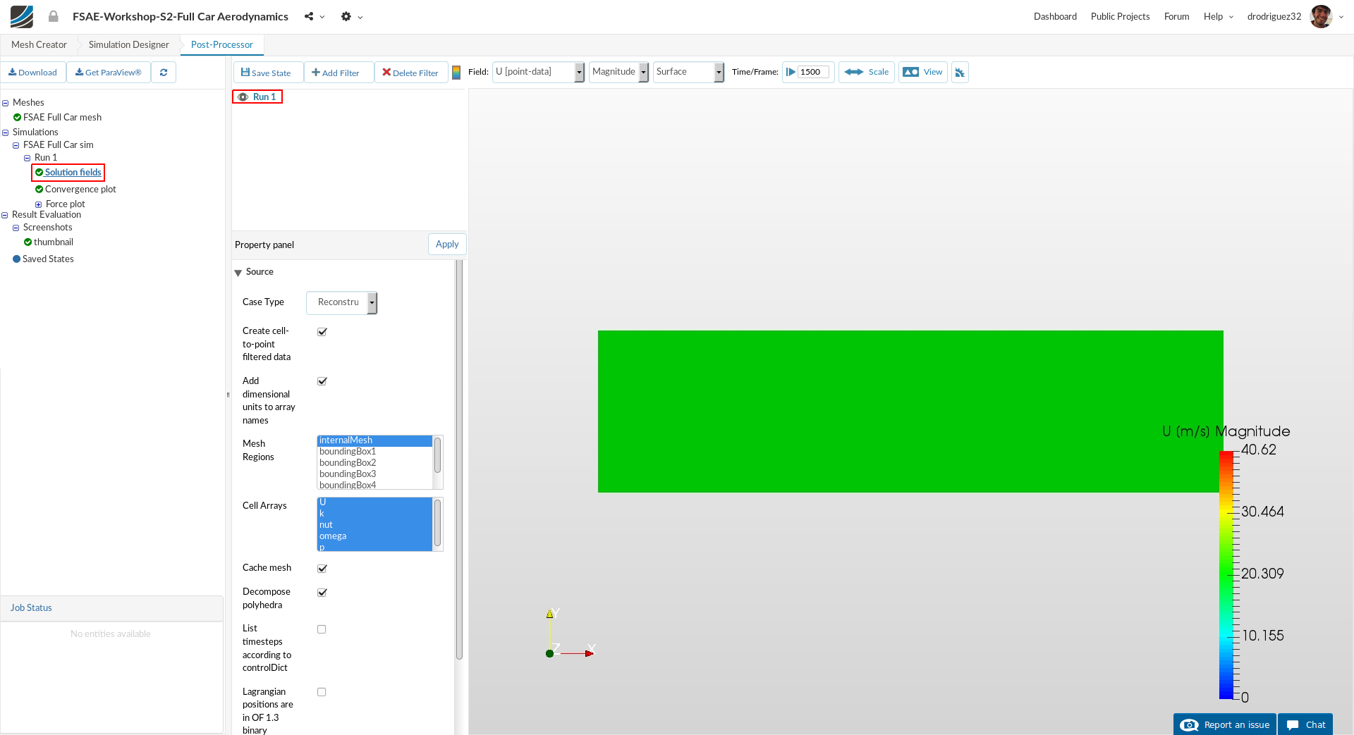
Once in Post-Processor, click on Solution fields under FSAE Full Car sim in order to load the results in viewer. Due to fine mesh it can take up to 5 minutes to load the results in to the viewer.
Slice 1

For faster and efficient reviewing of the results, we will use slice filter. In order to add the filter, do the following:
-
Go to Add Filter and select Slice.
-
Change Origin middle value (y value) to 0.0011
-
Change Normal to (0,1,0)
-
Uncheck Show Plane.
-
Click Apply to save the changes.
-
Next set camera orientation to +Y from the View tool over the viewer to get a proper view.
Slice 2
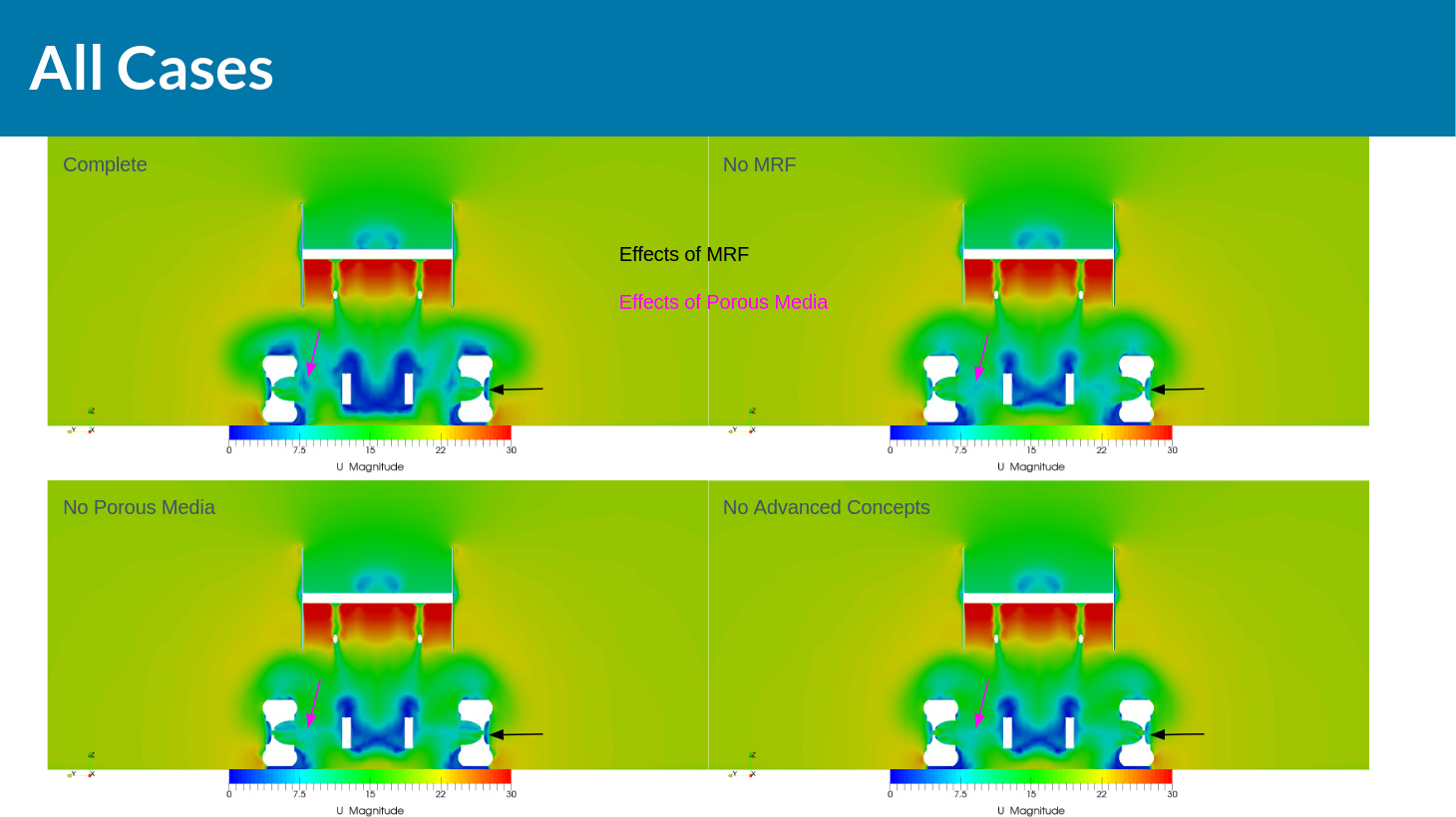
In order to see the pressure and velocity distribution on tires, we have to make another slice. This will be useful afterwards to compare the results between different configurations.
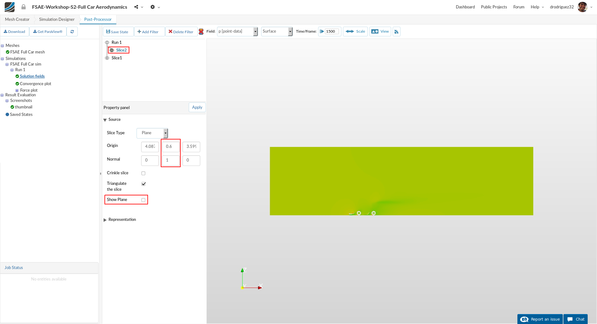
First go back to the actual solution field (Click on Run 1) and then:
-
Go to Add Filter and select Slice.
-
Change Origin middle value (y value) to 0.6
-
Change Normal to (0,1,0)
-
Click Apply to save the changes.
-
Turn off the previous created slice by unchecking the eye button next to it.
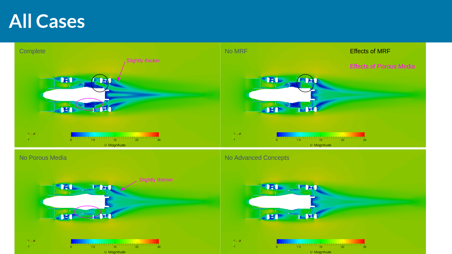
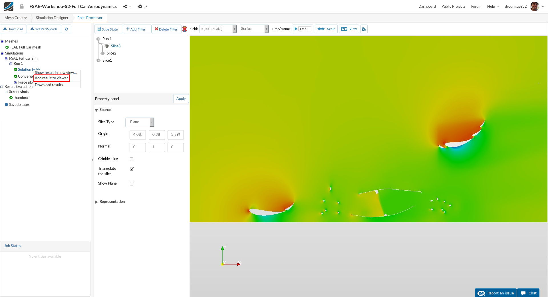
Slice - Pressure drop across radiator
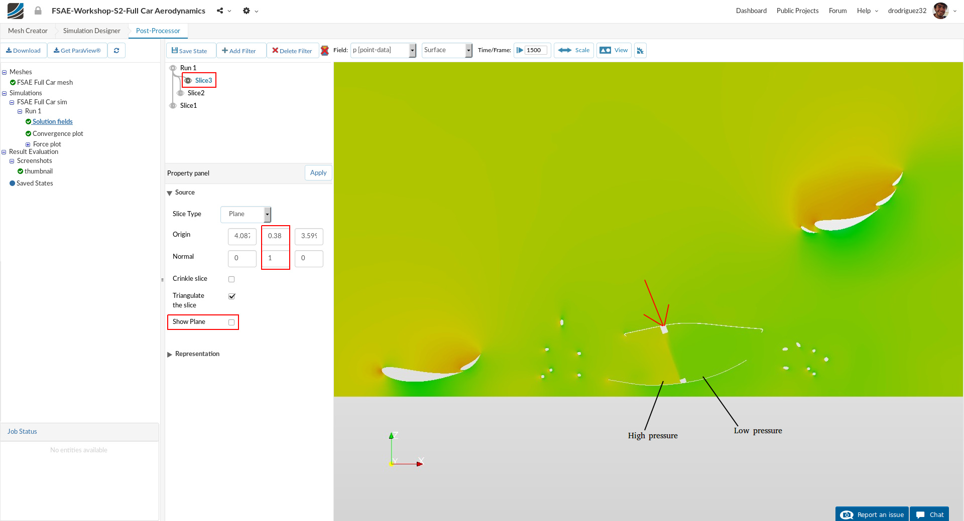
Go back to the actual solution field (Click on Run 1) and then:
-
Go to Add Filter and select Slice.
-
Change Origin middle value (y value) to 0.38
-
Change Normal to (0,1,0)
-
Click Apply to save the changes.
-
Turn off the previous created slices by unchecking the eye button next to it.
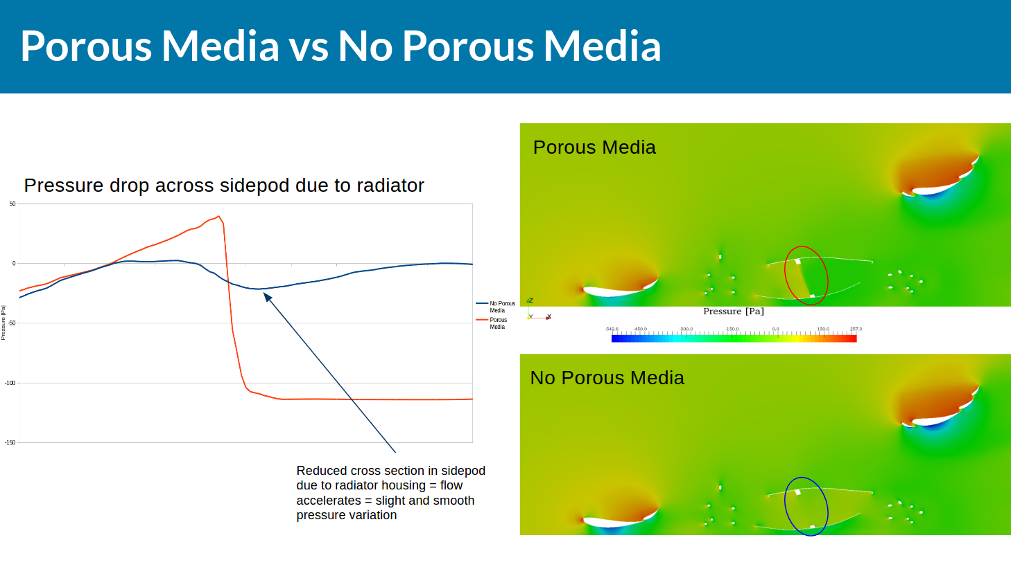
Notice how there is a pressure buildup in front of the radiator and a sudden pressure drop across it.
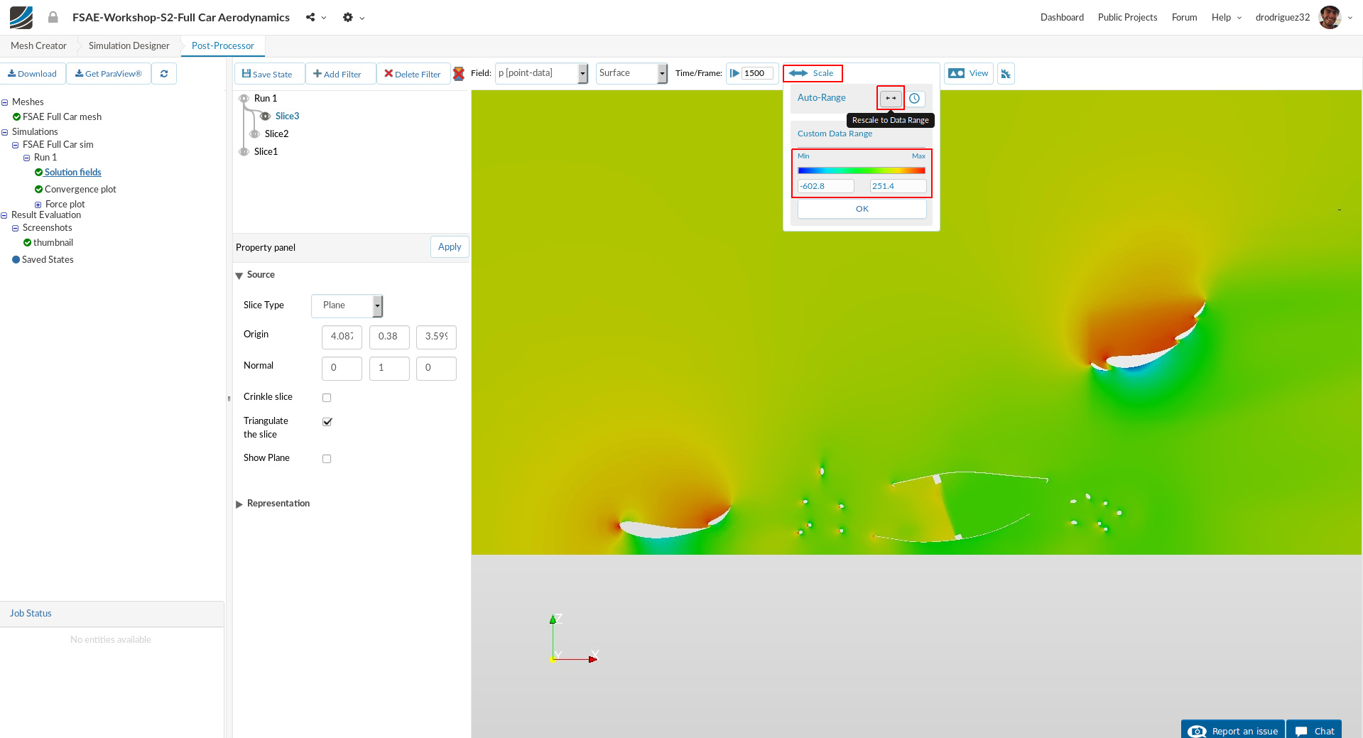
If you’re having trouble with the color distribution, click on Scale at the top and then on the arrows next to Auto Range.
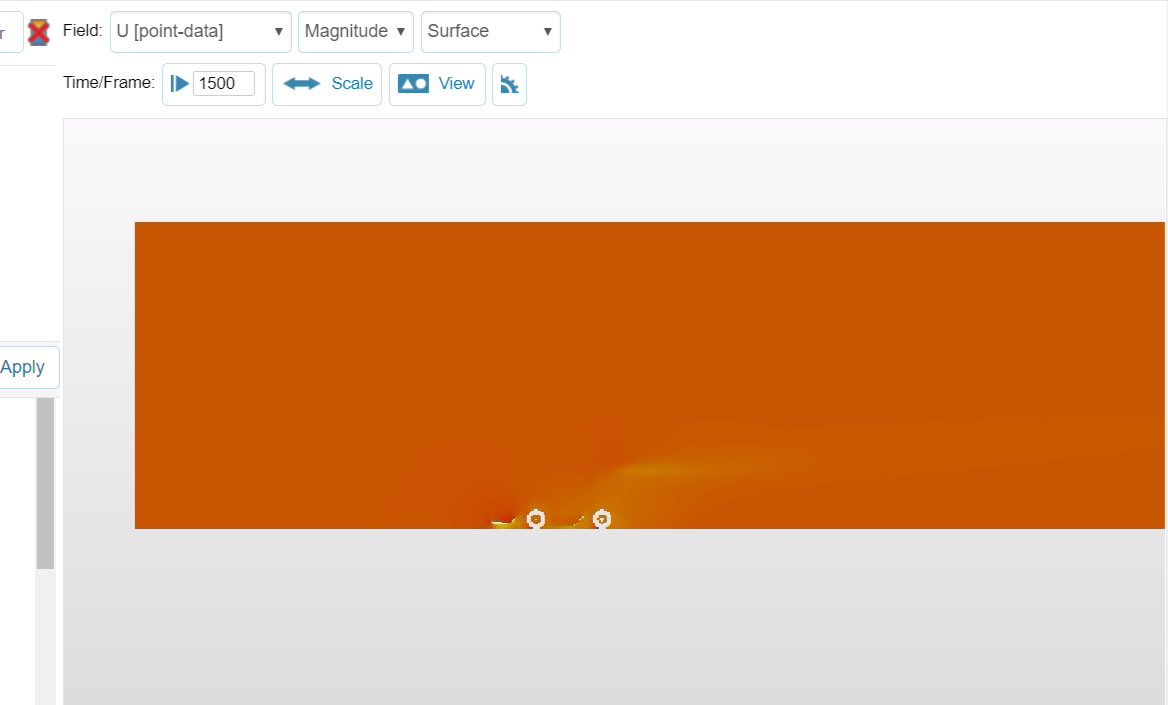
Slice - Velocity
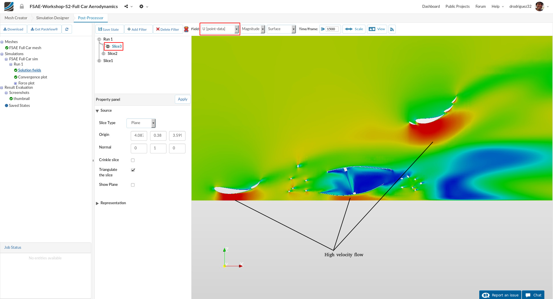
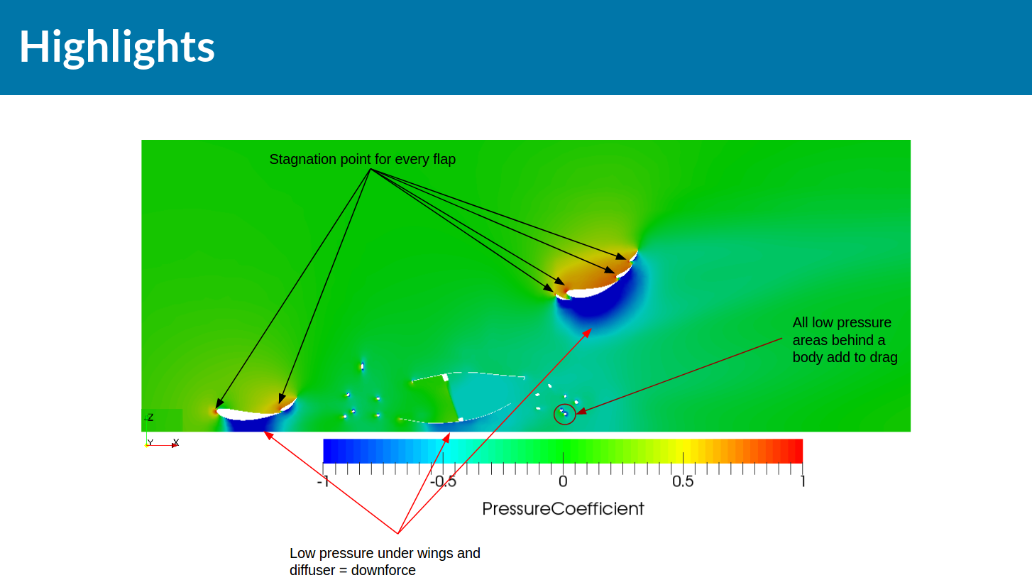
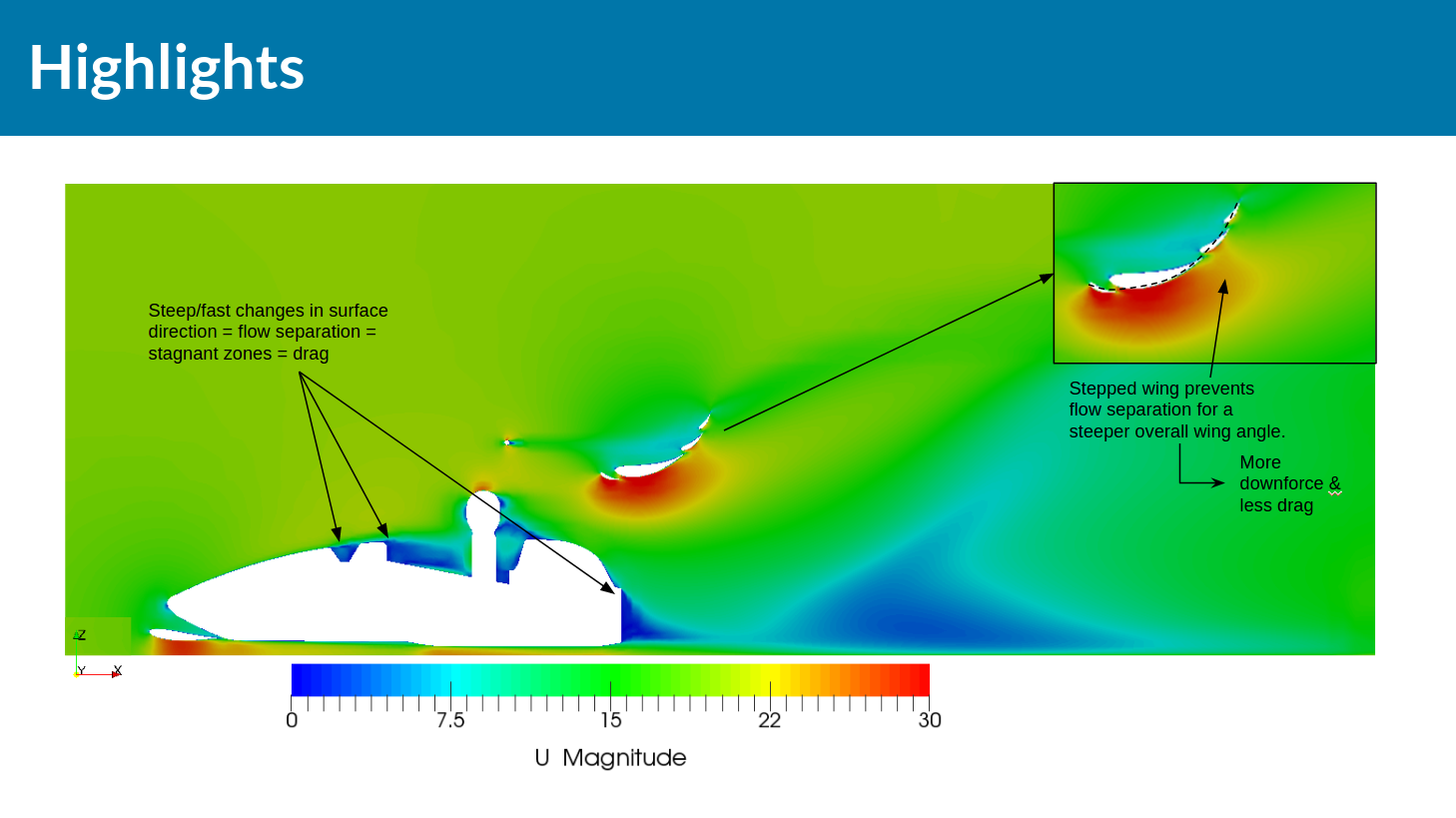
Another interesting field to visualize is the velocity. For the previous slice, change the field to U [point-data]. Note the high velocity flow below the wings - this is how they generate downforce. Also, notice that the flow becomes almost stagnant when it enters the sidepod and hits the radiator.
Visualize the Car
Now we will move further to load the whole car model in order to see the pressure contours over it.
For this load again the same result by right clicking on it and then selecting Add result to viewer.
Please note that adding second time the same results can take up to 10 min.
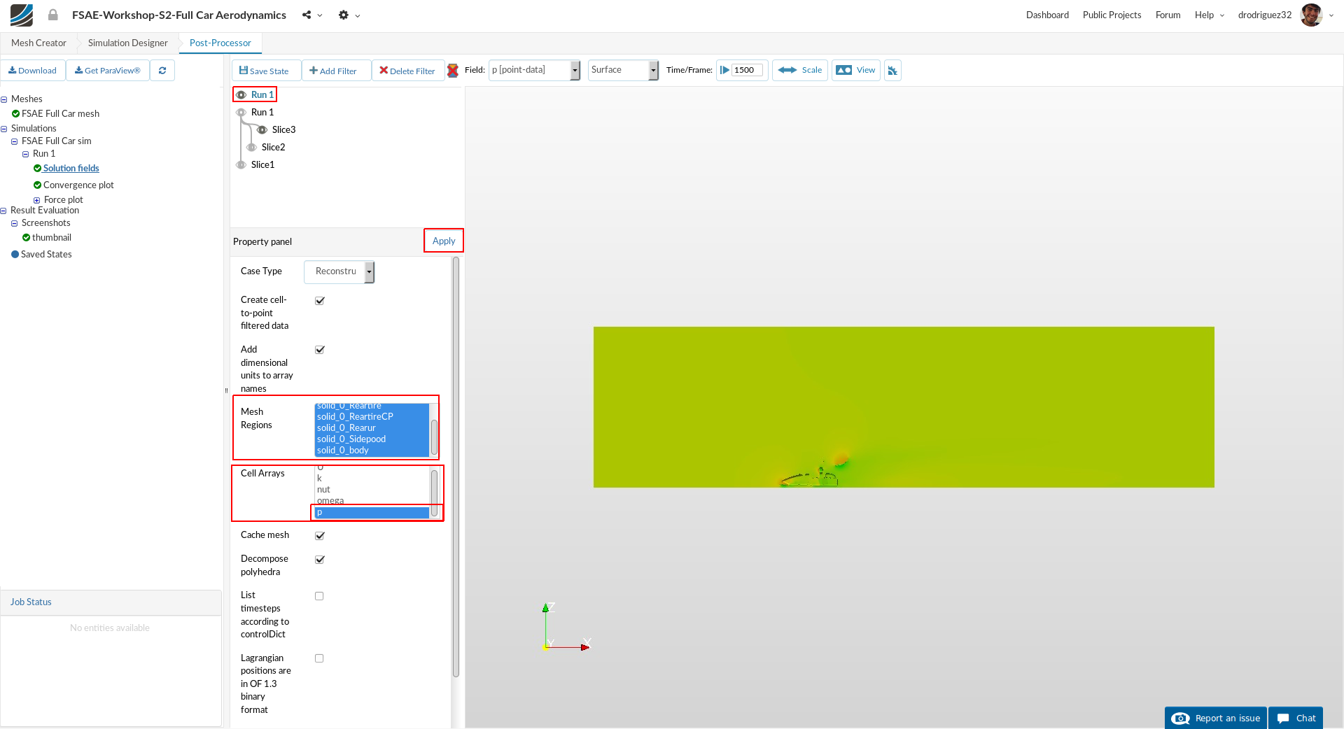
Once the results are loaded, select all the entities next to Mesh Regions starting with solid_0. You can do so by first selecting the first entry i.e. solid_0_body in this case and then holding shift button while going down and then selecting the last one. Next choose only p next to Cell Arrays. Click Apply to save the changes.
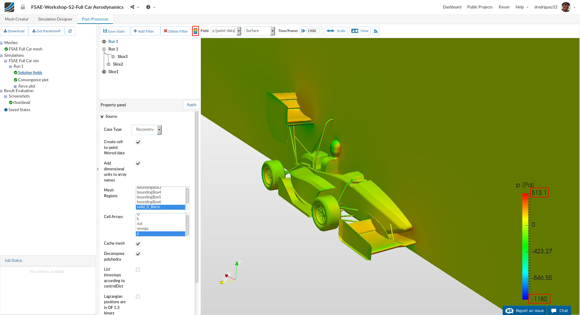
Turn on the color bar for pressure and turn on the view for Slice 1
Streamlines
Next we will create the stream lines in order to see the flow.
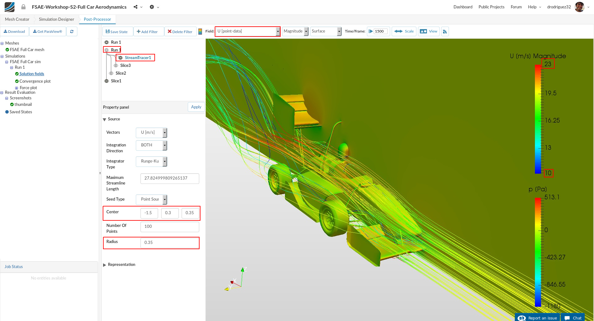
For this, go back to the first loaded result Run 1 (So the one that has all the slices)
-
Add a filter named StreamTracer
-
Change Center to (-1.5,0.3,0.35)
-
Change Radius to 0.35
-
Click Apply to see the streamlines.
-
Next switch to U [point-data] in order to see the streamlines colored via velocity.
As a last step, we have to rescale the velocity contour to a desired value. To do so, go to the Scale tool and give the lowest and highest values as 10 and 23 respectively. Then click OK. Now also turn on the color bar for the velocity by clicking the color bar button.
Homework Submission
Your homework is to investigate the Full car model FSAE Full Car with a radiator using the porous media approach, rotating wheels using the rotating wheel boundary condition, and rotation of the car rims using Multi Reference Frame (MRF). For this case, the front wing flap angle of 0 degrees will be considered and the velocity of the car will be set at a constant 20 m/s.
The step-by-step tutorial below contains all of the steps for setting up the simulation in SimScale and visualizing the results.
We’ve made an update to the platform and the sharing procedure has changed. Please go to the following link to see how to get a sharing link for your project:
New Sharing on SimScale
Homework Deadline: October 3rd, 11:59 pm CEST
Click Here to Submit your Homework
Recommendations About Comments
If you run into issues during your process, before adding a comment to the thread please consider the following:
- Go over the tutorial one last time and compare it to your setup. Is everything the same?
- Go over the existing comments. Maybe someone has had the same problem and it’s already solved.
- Is there an actual error? Or is it taking a long time to load?
a. If it seems to be a loading issue, please give it some time or refresh the page. Sometimes due to the internet connection the platform may seem slow.
If it’s a new issue that you can’t solve, please outline the issue as specifically as possible and include a link to your project. This will help us figure out what is going on faster and thus we can get back to you faster.