Recording
Pictures
If you have trouble enlarging the pictures in the tutorial, you can find them here:
Pictures
Introduction
As the focus of these workshops is an advanced aerodynamic setup for your car, we are assuming that you are familiar with the CFD concepts mentioned during the tutorial. For those of you who are unfamiliar with MRF zones, Porous zones, or Rotating Wall boundary conditions, it is recommended that you go over the following links:
- 2017 FSAE Workshop - Session 2 (Part 1) and 2017 FSAE Workshop - Session 2 (Part 2)
- SimScale Documentation - Rotating Zones
- SimScale Documentation - Rotating Wall Boundary Condition
- SimScale Documentation - Porous Media
Focus of the tutorial
For this tutorial we will study an FSAE car moving forward at a constant 20 \frac{m}{s}. We will investigate the effect of changing the rake angle of the car by lowering the nose or lowering the rear. Here you will find the setup for the standard ride height - the setup of the different models will be exactly the same.
Measuring Ride Height
In the project you import you will find the following 5 models:
| Model Name | Front Height [mm] | Rear Height [mm] | Rake Angle [^{\circ}] |
|---|---|---|---|
| Standard | 55.72 | 55.72 | 0 |
| Low Nose | 40 | 55.72 | 0.6 |
| Low Nose 2 | 25 | 55.72 | 1.1 |
| Low Rear | 55.72 | 45 | -0.4 |
| Low Rear 2 | 55.72 | 30 | -0.9 |
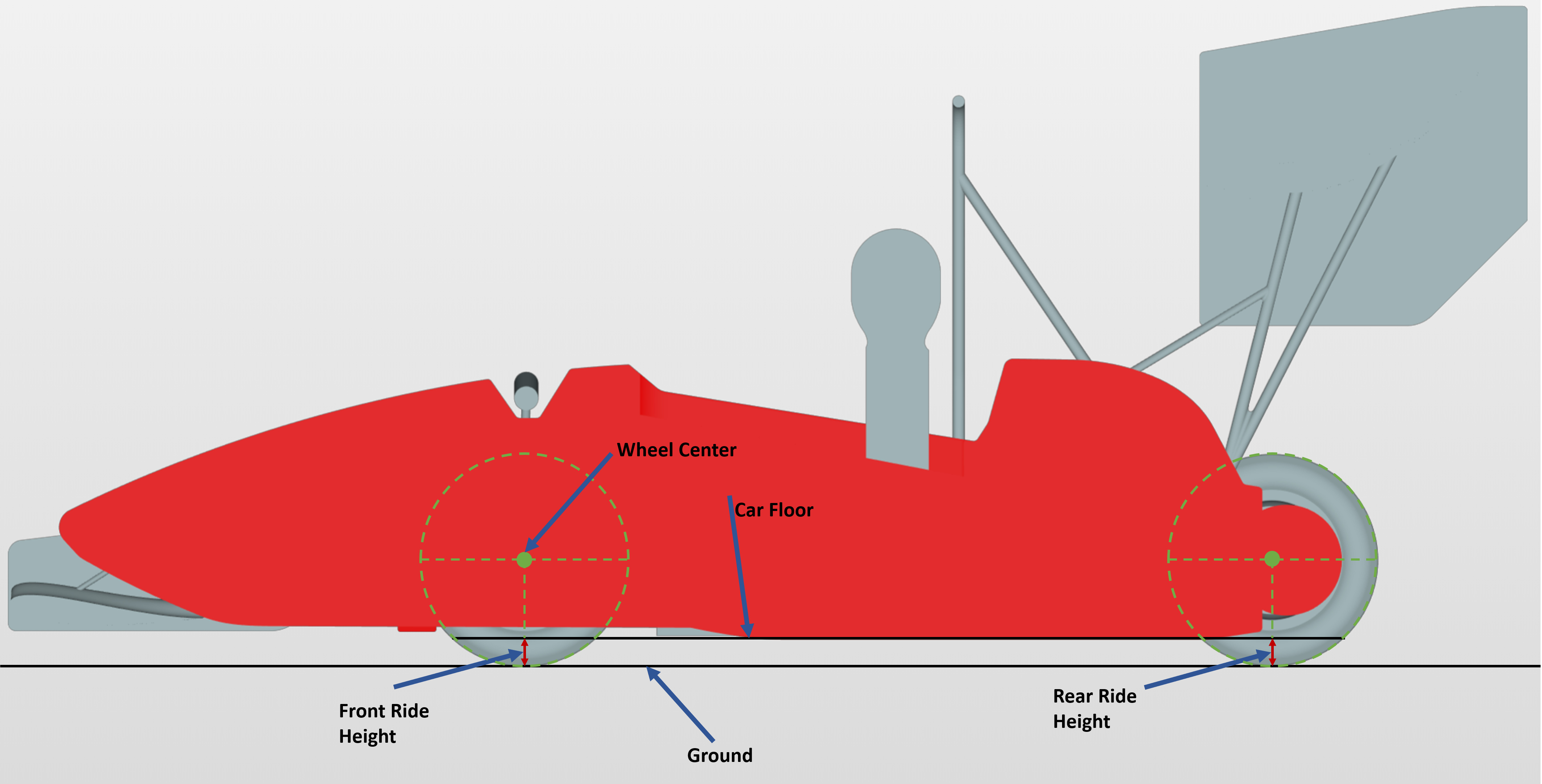
To measure the ride height of our car we have used an approach commonly used in F1. Due to the stepped floor we have a higher reference at the front wheels, and due to the length of the wheel base, we don’t have a physical floor at the center of the rear wheels. So what we do is draw a plane at the lowest step of the floor, and measure the vertical distance between that plane and the ground at the center of the front wheels and the rear wheels. It is better illustrated in the image below.
Project Import
To start this exercise, please import the project into your workspace by clicking on the link below:
FSAE Trackside Aerodynamics - Ride Height Analysis
Please make a copy to be able to work on it.
Mesh Generation

In the Mesh Creator tab, click on the geometry FSAE-Standard and click on New Mesh to start creating a new mesh.
The new mesh operation will be generated automatically.
Next change:
-
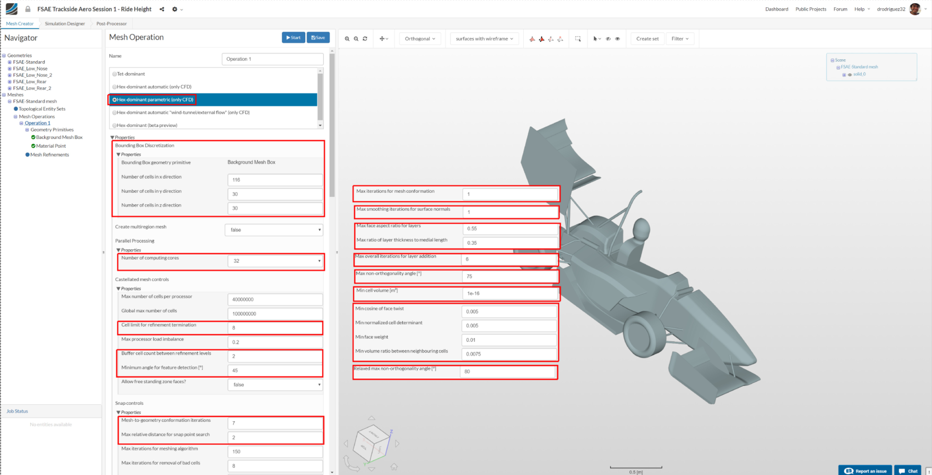
Type to Hex-dominant parametric (only CFD)
-
Bounding Box geometry primitive to the following:
Number of cells in x direction to 116
Number of cells in y direction to 30
Number of cells in z direction to 30 -
Number of parallel computing cores to 32 Scroll down to change other values to optimize the meshing parameters
-
Cell limit for refinement termination to 8
-
Buffer cell count between refinement levels and Minimum angle for feature detection [°] to 2 and 45 respectively
-
Mesh-to-geometry conformation iterations to 7, Max relative distance for snap point search to 2, and Max iterations for mesh conformation to 1
-
Max smoothing iterations for surface normals [-] to 1
-
Max face aspect ratio for layers [-] and Max ratio of layer thickness to medial length [-] to 0.55 and 0.35 respectively
-
Max overall iterations for layer addition to 6
-
Max non-orthogonality angle to 75
-
Min cell volume [m^3] to 1e-16
-
Min cosine for face twist, Min normalized cell determinant,Min face weight and Min volume ratio between neighbouring cells to 0.005, 0.005, 0.01 and 0.0075 respectively
-
Relaxed max non-orthogonality angle to 80
-
Click Save to register changes.
Geometry Primitves
Background Mesh Box
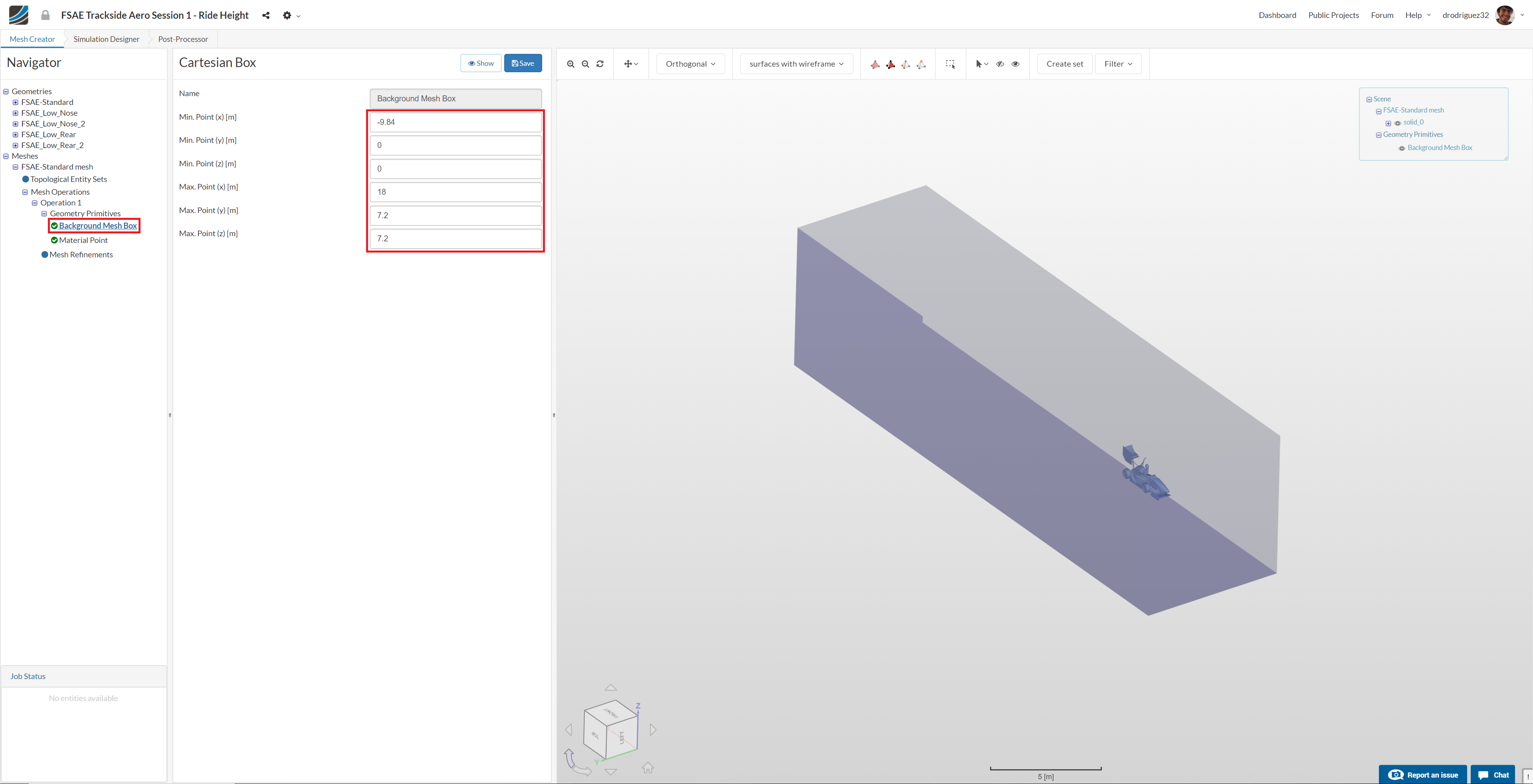
Go to Background Mesh Box under Geometry Primitives and change the mesh box dimensions:
Min. Point (x) = - 9.8
Min. Point (y) = 0
Min. Point (z) = 0
Max. Point (x) = 18
Max. Point (y) = 7.2
Max. Point (z) = 7.2
Click Save to save the changes. Click on reset icon over viewer to see the created mesh box in viewer.
MaterialPoint

Go to MaterialPoint and change the values to the following:
Center (x) = 0
Center (y) = 2
Center (z) = 2
Then click Save
Cartesian Box - Lower
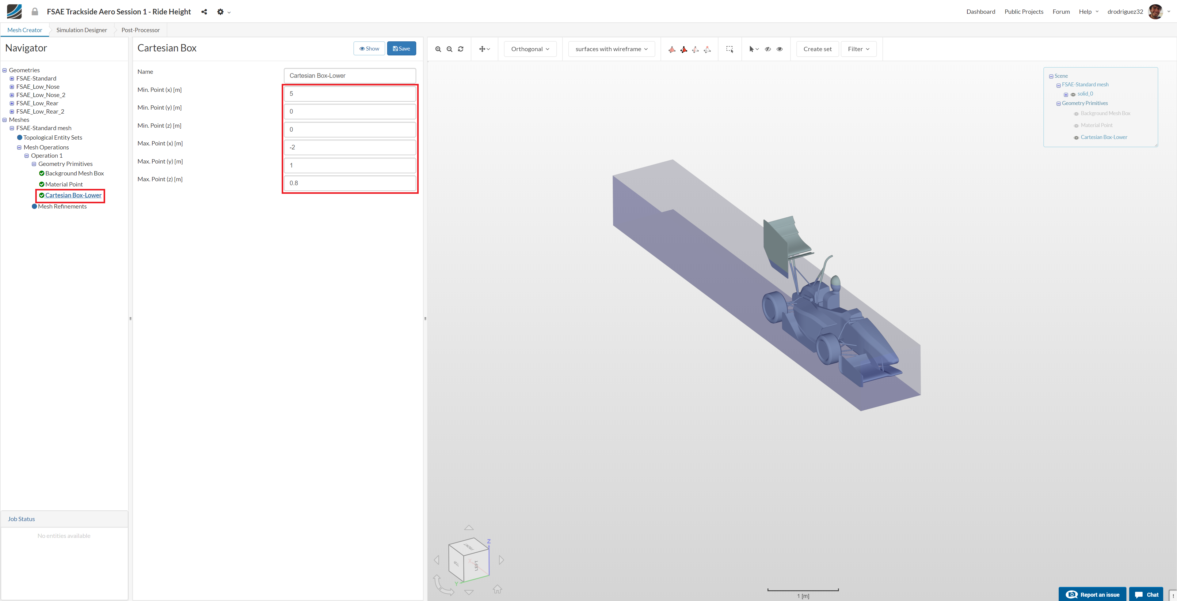
After creating a new Cartesian Box, you will be directed to the definition of this Cartesian Box. Rename it to Cartesian Box-lower (optional) and change the dimensions of the box to the following:
Min. Point (x) = 5
Min. Point (y) = 0
Min. Point (z) = 0
Max. Point (x) = - 2
Max. Point (y) = 1
Max. Point (z) = 0.8
This box will be refined later in the process and it will allow us to get better results and observe with more detail the flow around the car and directly in its wake.
Click Save to register your changes.
Cartesian Box - Upper

Create another Cartesian Box for further refinement definitions and rename it to Cartesian Box-upper (optional). This time change the values to the following:
Min. Point (x) = - 0.4
Min. Point (y) = 0
Min. Point (z) = 0.8
Max. Point (x) = 5
Max. Point (y) = 0.7
Max. Point (z) = 1.6
Like the past one, this will also be refined and allow us to get better results around the back wing and better observe its wake.
Click Save to register your changes.
Mesh Refinements
A good mesh requires well defined refinements. Now we will start creating the mesh refinements. For this proceed to Mesh Refinements and click +New
Mesh Refinement 1 - Surface
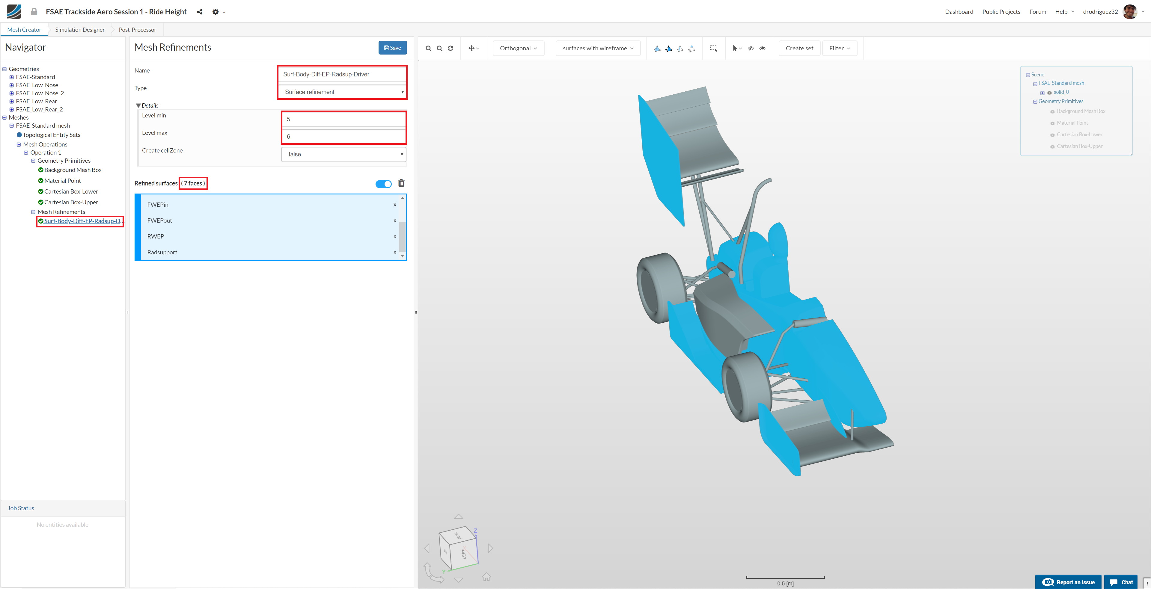
A new mesh refinement will be created. Rename it to Surf-body-diff-EP-Radsup-Driver (optional).
Change the Type to Surface refinement and change Level min and Level max to 5 and 6 respectively.
From the navigator in the right select body, FWEPin (Front Wing Inner Endplate), FWEPout (Front Wing Outer Endplate), RWEP (Rear Wing Endplate), Diffuser, Radsupport and Driver
You should see those faces under Refined surfaces (7 faces) and they should be highlighted in blue.
Click Save to register your changes.
Mesh Refinement 2 - Surface
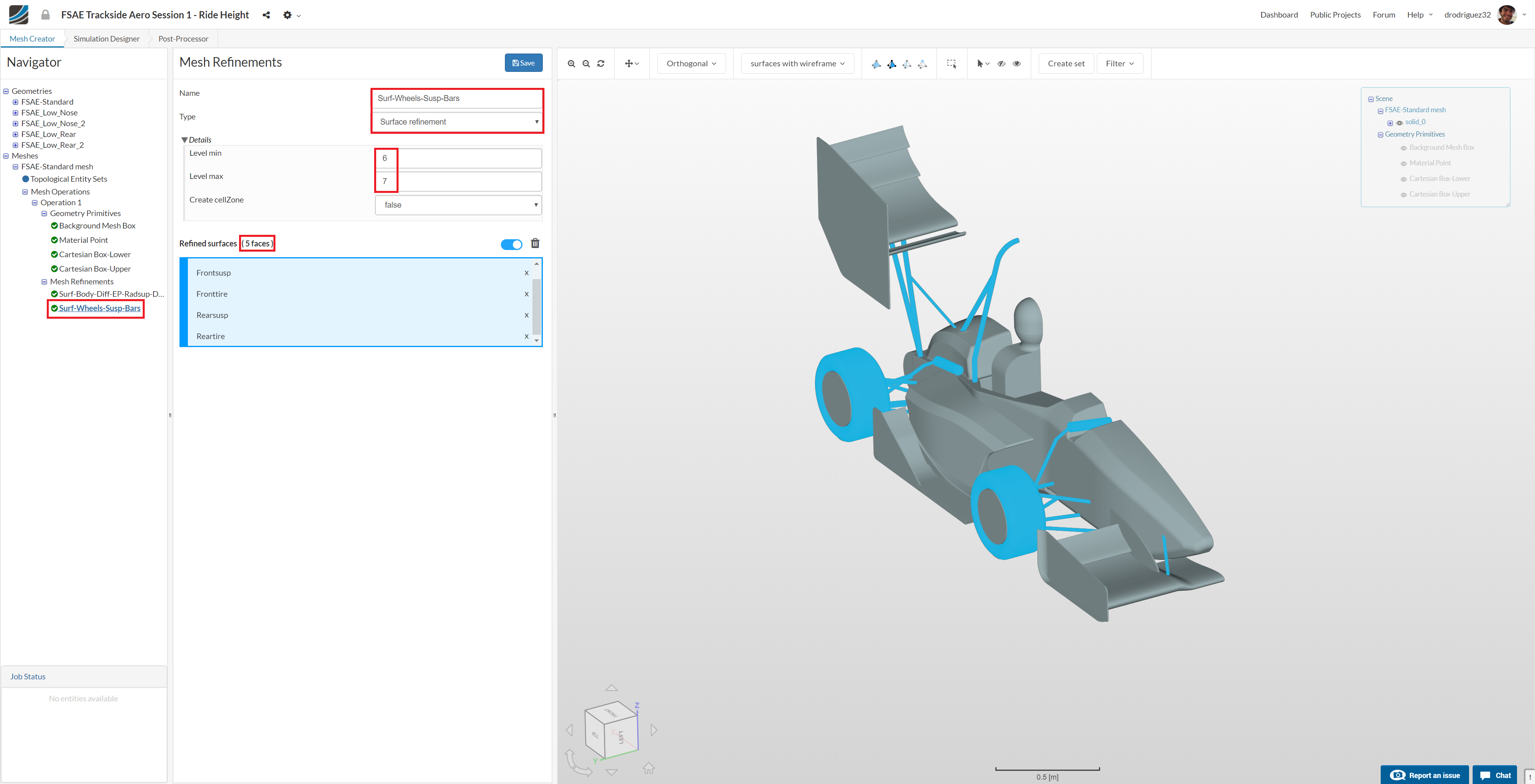
Create a new mesh refinement and rename it to Surf-wheels-susp-bars (optional).
Change the Type to Surface refinement and change Level min and Level max to 6 and 7 respectively.
From the navigator in the right select Frontsusp, Rearsusp, Barre, Reartire and Fronttire.
You should see those faces under Refined surfaces (5 faces) and they should be highlighted in blue.
Click Save to register your changes.
Mesh Refinement 3 - Surface
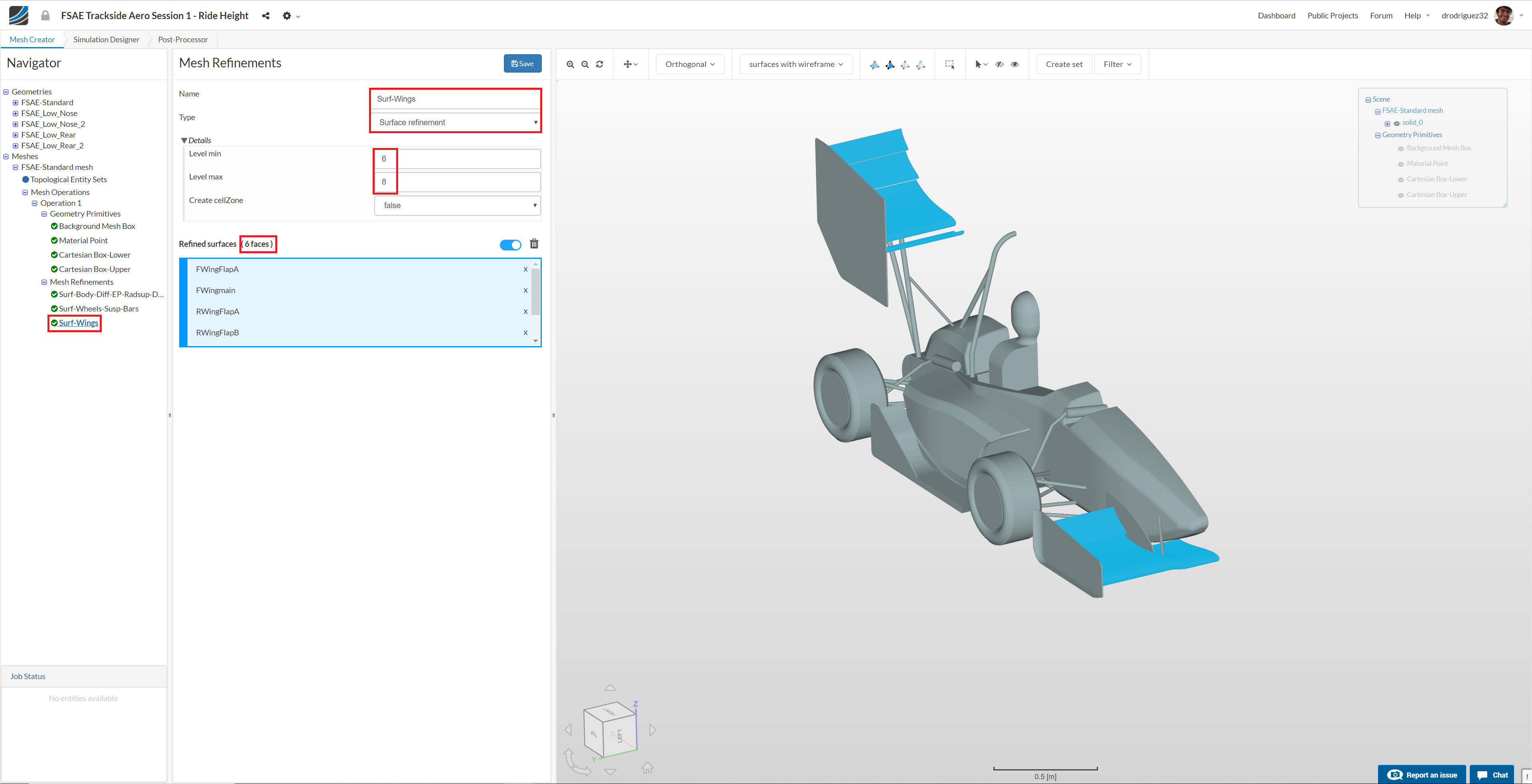
Create a new mesh refinement and rename it to Surf-wings (optional).
Change the Type to Surface refinement and change Level min and Level max to 6 and 8 respectively.
From the navigator in the right select FWmainwing, FWflap, RWflapa, RWflapb, RWflapc, RWflapd.
You should see those faces under Refined surfaces (6 faces) and they should be highlighted in blue.
Click Save to register your changes.
Mesh Refinement 4 - Surface
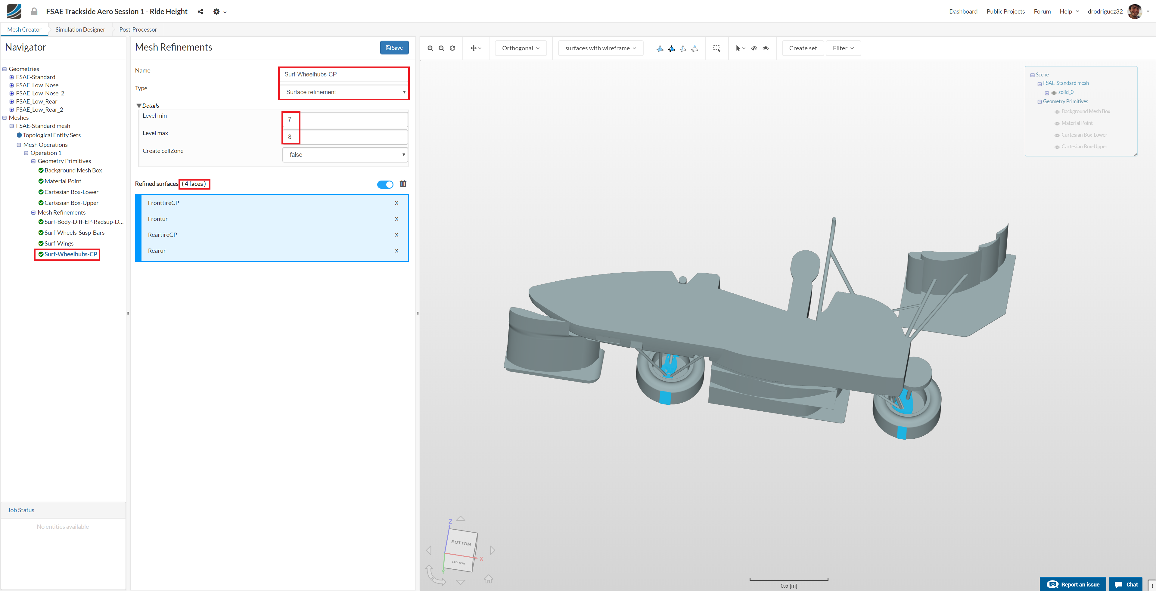
Create a new mesh refinement and rename it to Surf-Wheelhubs-CP (optional).
Change the Type to Surface refinement and change Level min and Level max to 7 and 8 respectively.
From the navigator in the right select Frontur, Rearur, ReartireCP and Fronttirecp
You should see those faces under Refined surfaces (4 faces) and they should be highlighted in blue.
Click Save to register your changes.
Mesh Refinement 5 - Surface
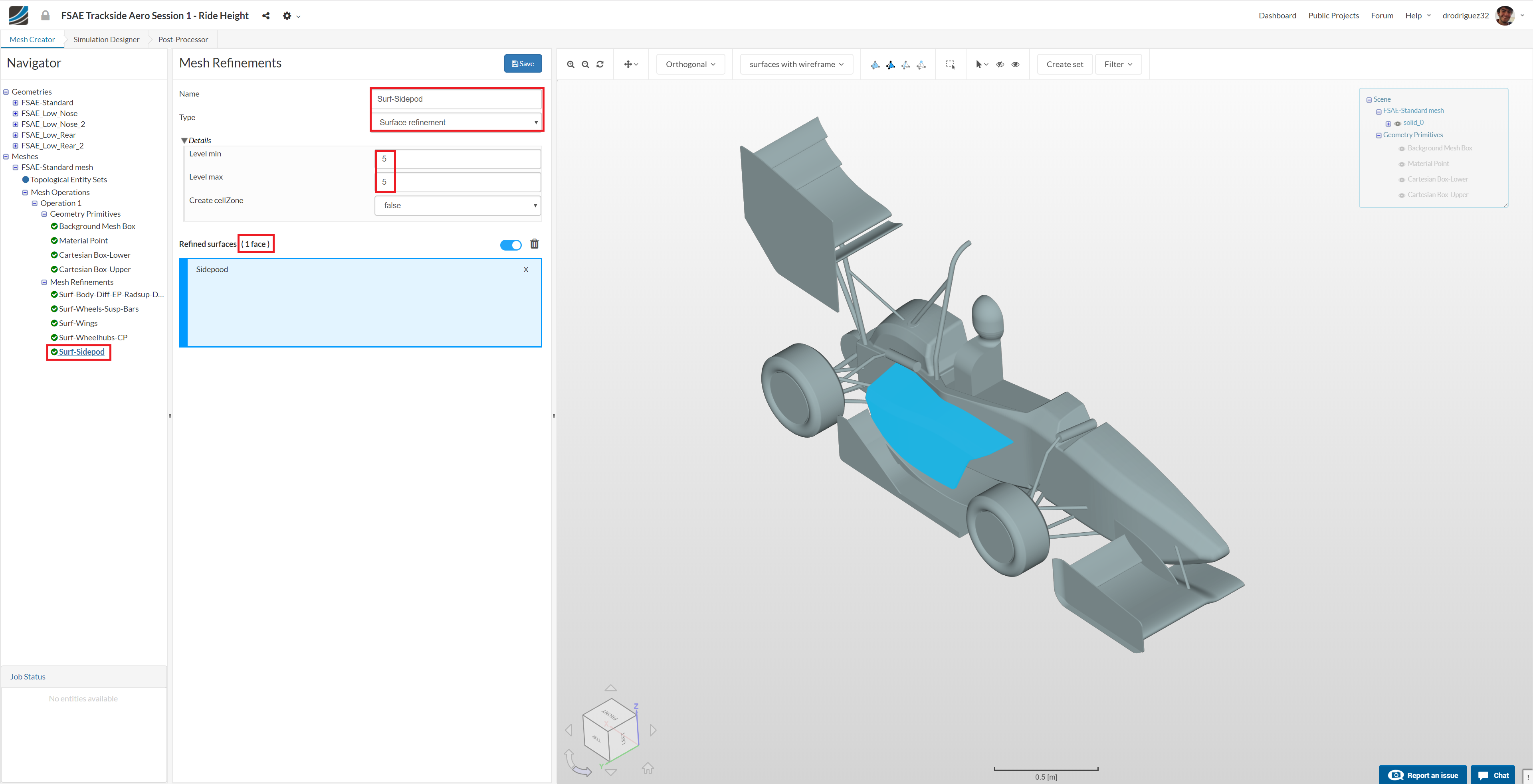
Create a new mesh refinement and rename it to Surf-Sidepod (optional).
Change Type to Surface refinement and change Level min and Level max to 5 and 5 respectively.
From the navigator in the right select Sidepod
You should see the face under Refined surfaces (1 face) and it should be highlighted in blue.
Click Save to register your changes.
Mesh Refinement 6 - Rotating Zone
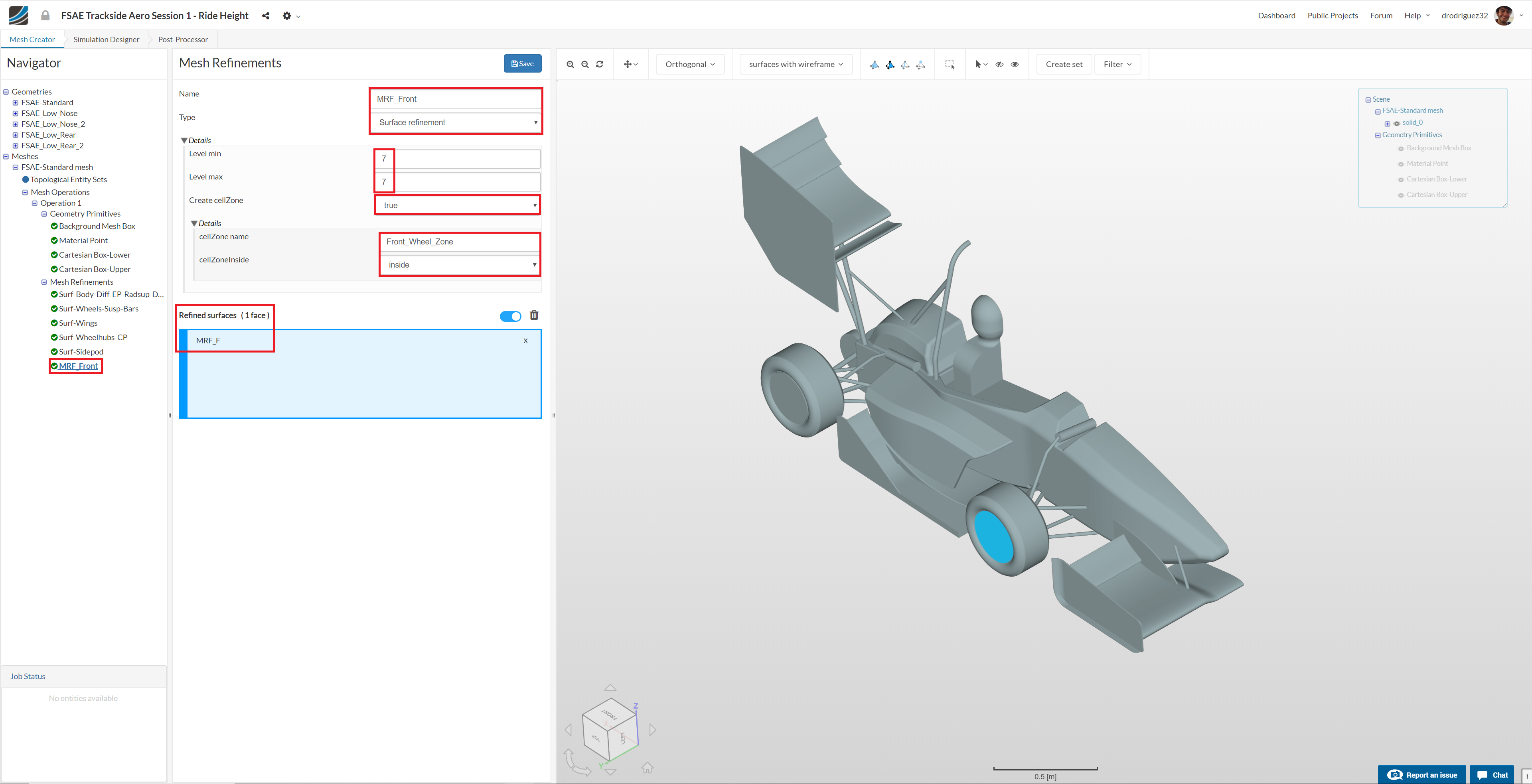
Create a new refinement and rename it to MRF-Front (optional).
Change the Type to Surface refinement and change both Level min and Level max to 7 respectively.
Change Create cellZone to true and rename cellZone name to Front_Wheel_Zone
Select MRF_F
Click Save to register your changes.
Mesh Refinement 7 - Rotating Zone
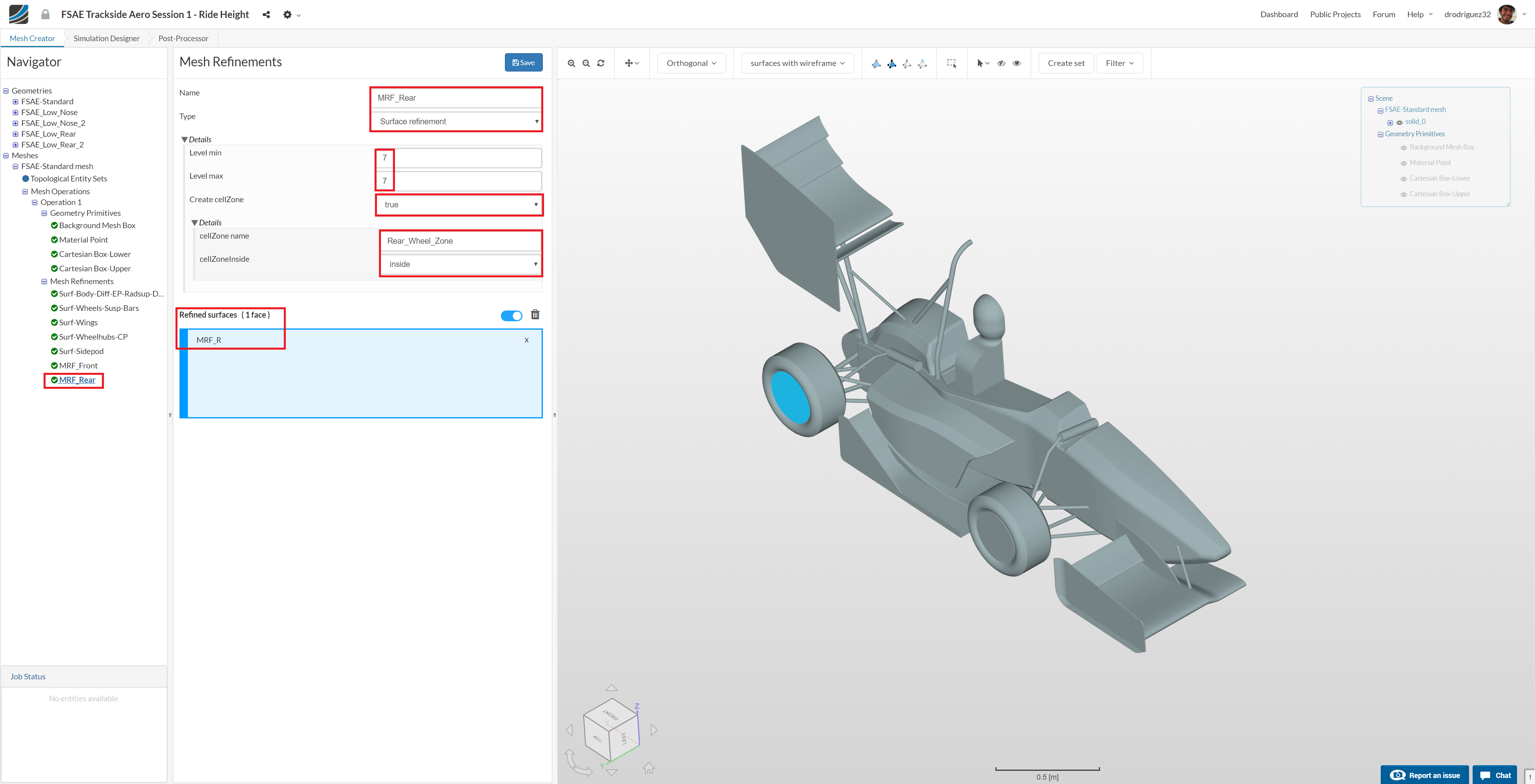
Similarly, for the rear MRF create a new mesh refinement and rename it to MRF-Rear (optional).
Change the Type to Surface refinement and change both Level min and Level max to 7 respectively.
Change Create cellZone to true and rename cellZone name to Rear_Wheel_Zone
Select MRF_R
Click Save to register your changes.
Mesh Refinement 8 - Porous Zone
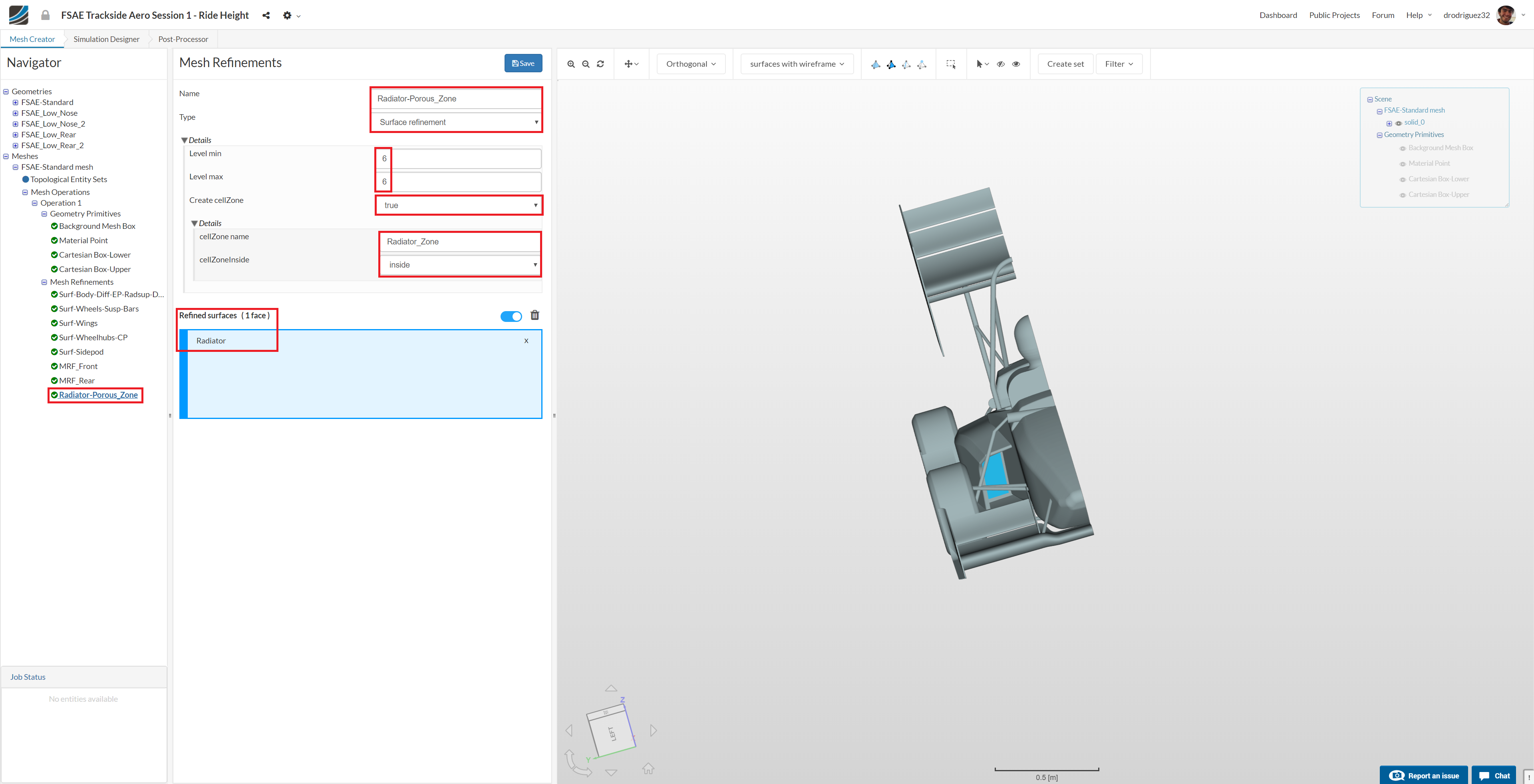
Create a new mesh refinement and rename it to Radiator-Porous-Zone (optional).
Change Type to Surface refinement and change Level min and Level max to 6 and 6 respectively.
Change Create cellZone to true and rename cellZone name to Radiator_Zone
From the navigator in the right select Radiator
You should see the face under Refined surfaces (1 face) and it should be highlighted in blue.
Click Save to register your changes.
Mesh Refinement 9 - Region

In order to define the refinement level for the created Cartesian boxes, create a new mesh refinement and rename it to Region (optional).
Change the Type to Region refinement and then change Feature refinements levels Level to 3. Select Cartesian Box-lower and Cartesian Box-upper under Geometry Primitives
Click Save to register the refinements for the specific Cartesian Boxes.
Mesh Refinement 10 - Boundary Layer
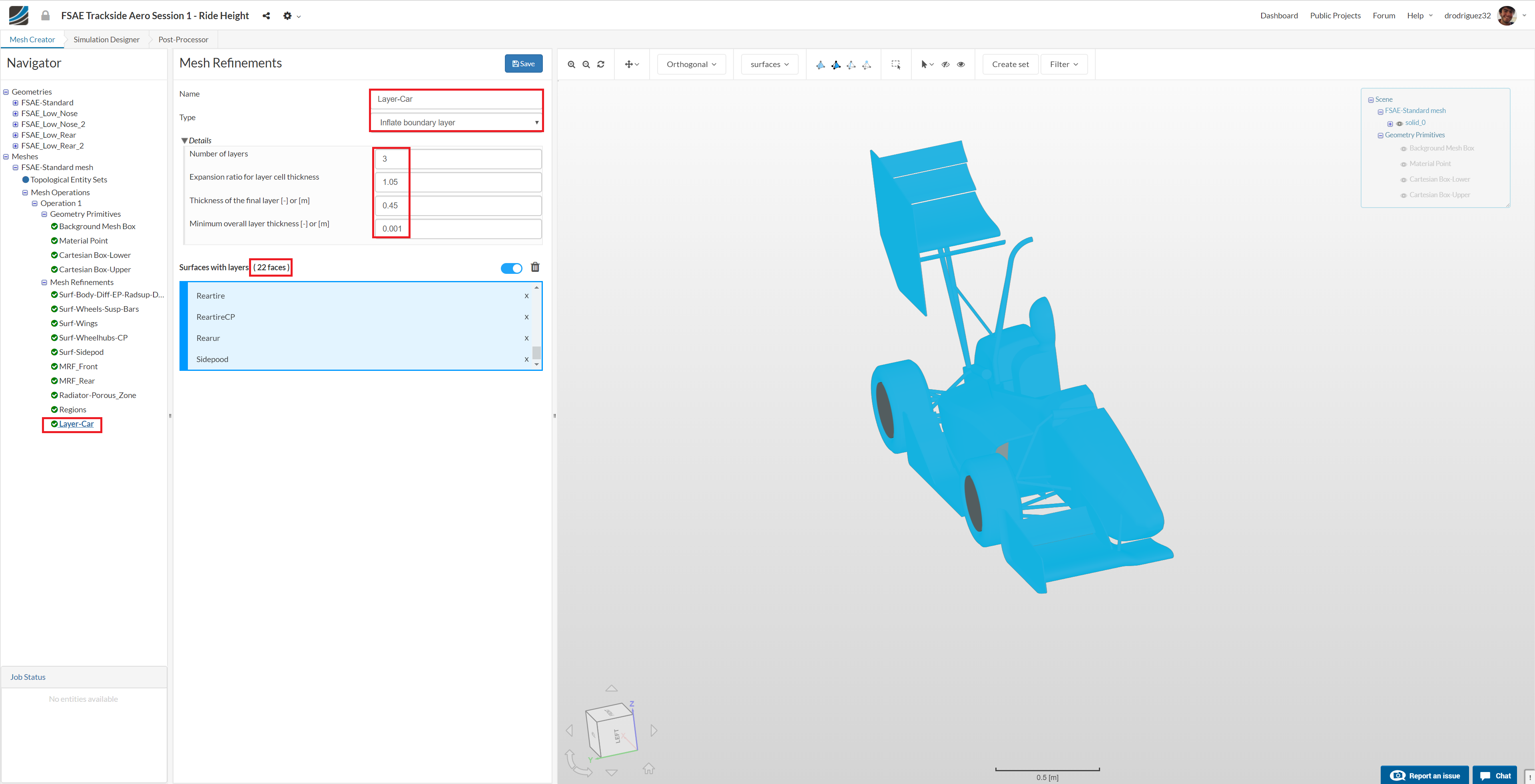
Create a new refinement and rename it to Layer-Car (optional).
Change the Type to Inflate boundary layer and further change Number of layers [-], Expansion ratio for layer cell thickness [-], Thickness of the final layer [-] and Minimum overall layer thickness [-] to 3 , 1.05, 0.45 and 0.001 respectively.
Select all the faces except Radiator; Radsupport, MRF_F and MRF_R.
You should have 22 faces selected.
Click Save to register your changes.
Mesh Refinement 11 - Boundary Layer

For the floor layers, create a new refinement and rename it to Floor-layer (optional).
Change the Type to Boundary box layer addition
Change Bounding box face to Zmin and then the Number of layers and Minimum overall layer thickness [-] to 3 and 0.001 respectively.
Click Save to register your changes.
Mesh Refinement 12 - Feature

In order to create a separate feature refinement for small features, create a new mesh refinement and rename it to Feat (optional).
Change Type to Feature refinement and then click + button to add an extra value. In the first row, change Distance and Level value to 0.001 and 8 respectively. Similarly, change the value to 0.005 and 6 in second row.
Click Save to save the feature refinement.
Start Mesh Operation
Once you have defined all of the mesh refinements, go back to the Operation 1 and click Start in order to submit the meshing job to the server. Due to the fineness of the mesh, the meshing could take 30 minutes to finish.
Simulation Setup
Once the meshing of the first geometry is finished, you can proceed to Simulation Designer

Once you are in Simulation Designer, click New Simulation. Under Fluid Dynamics choose incompressible and click on Create.
Domain
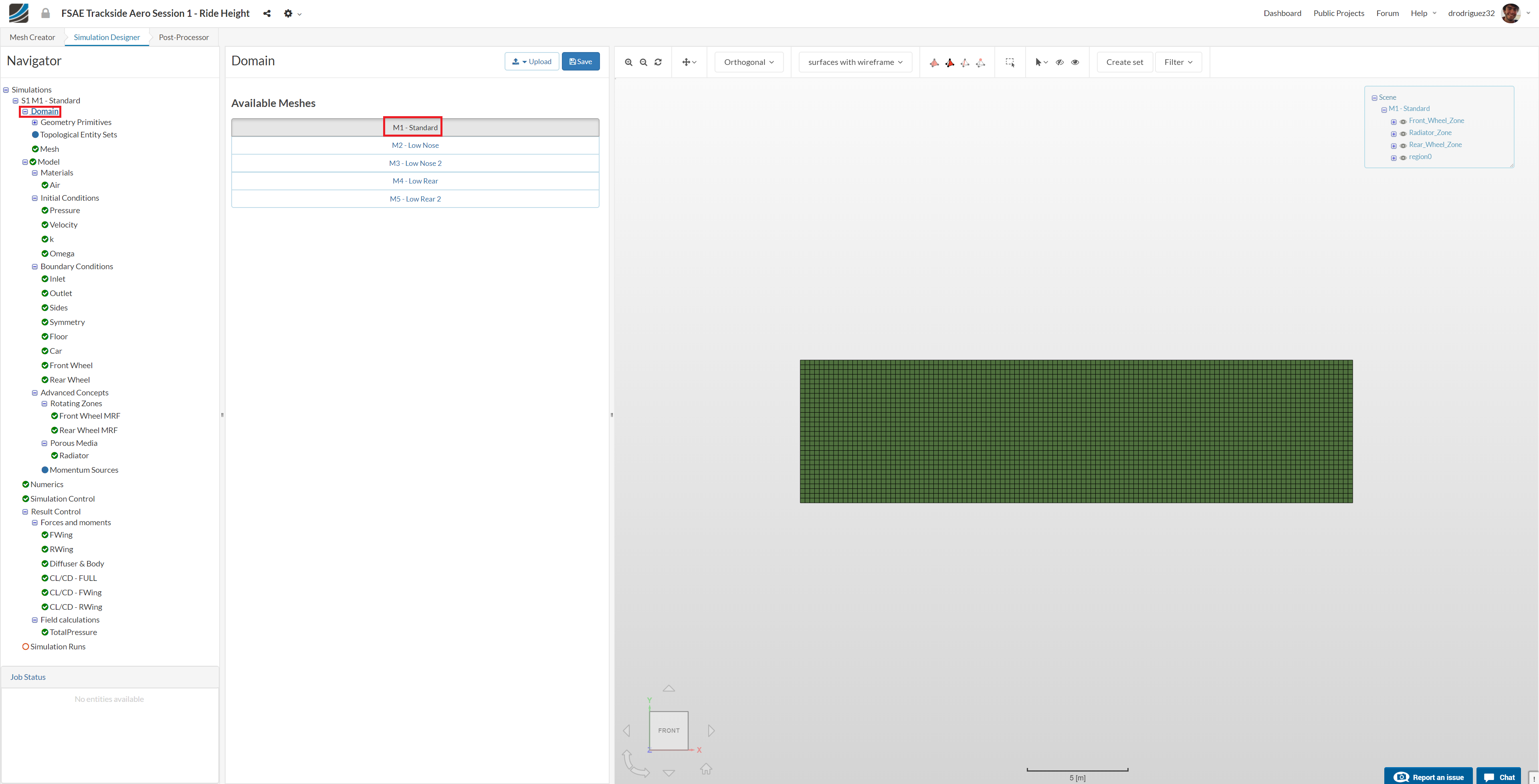
Next you have to select a domain on which this simulation will be performed. Proceed to Domain and select FSAE Standard mesh and click Save. After a while you will see the loaded mesh of the selected domain in the viewer. For the easier mesh handling, it is recommended to switch to surfaces render mode in the top viewer bar
Material

Under Material click New to create a new material. Then click Import from material library and select Air.
Select region0, Radiator_Zone, Front_Wheel_Zone and Rear_Wheel_Zone from the navigator in the right. You should see the list in the blue highlighted zone under Assignment.
Initial Conditions
We will now proceed to change the initial conditions. We will leave Pressure and Velocity with the defaults set by SimScale.

Go to k and change the Turbulent kinetic energy value [m²/s²] value to 0.06 and click Save.

Next go to Omega and change Specific turbulence dissipation rate [1/s] to 44.7 and click Save.
Boundary Conditions
Now we will proceed to the most crucial and important section of the simulation setup: setting up the boundary conditions. This is simply telling the platform how we want the simulation to behave.
Go to Boundary Conditions and click +New in order to create a new boundary condition.
Inlet
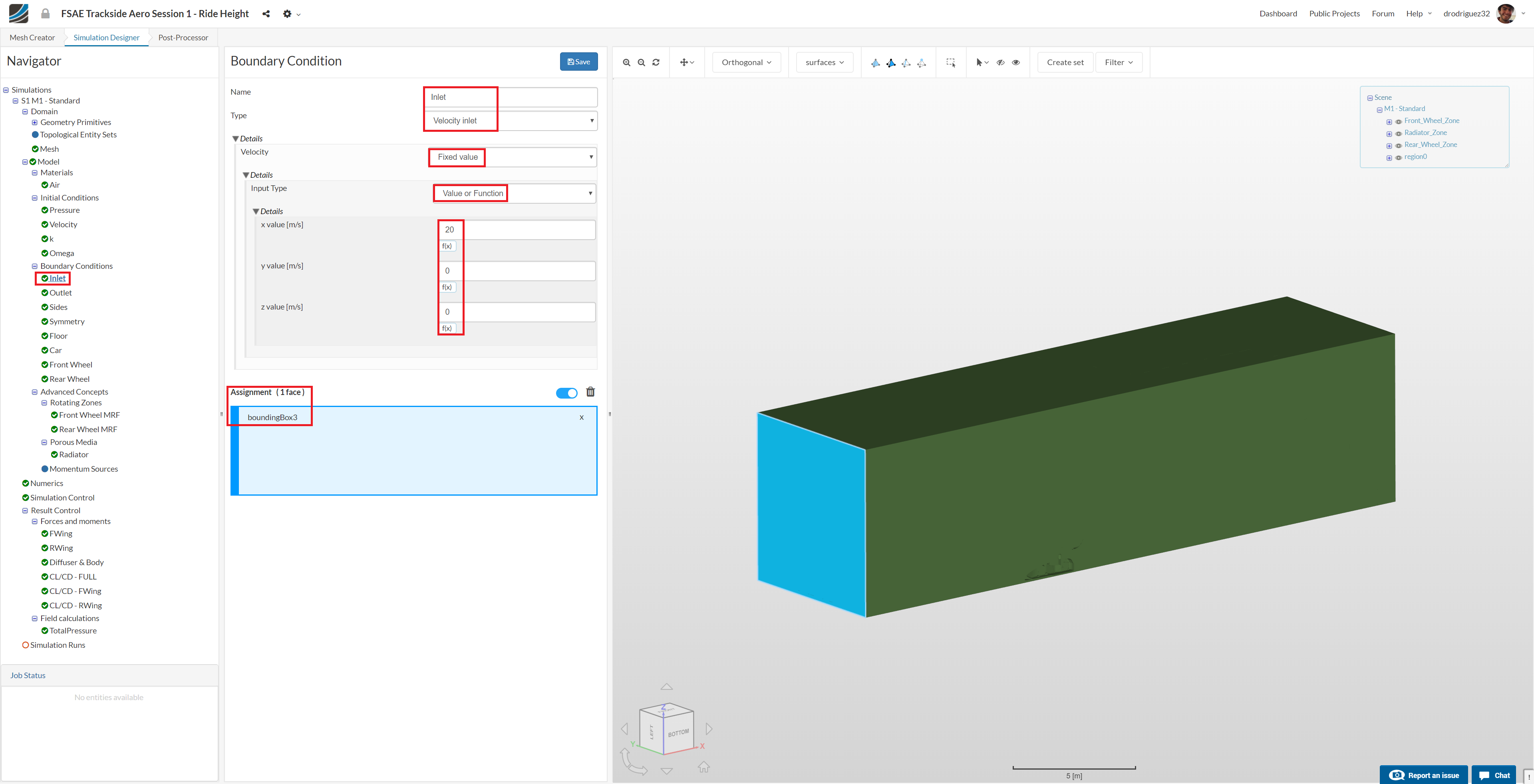
Rename the newly created boundary condition to Inlet (optional).
Set the Type to Velocity Inlet
Change x value [m/s] of Velocity to 20
Select the face of the bounding box that is before the car (boundingBox3). You can do this by clicking on it or simply selecting it from the navigator in the right.
Click Save to define the inlet boundary condition.
Outlet

Create a new Boundary Condition and rename it to Outlet (optional).
Change the Type to Pressure Outlet
Select boundingBox4 (the back face of the bounding box) from the navigator on the right or by clicking on the face.
Click Save to define the outlet boundary condition.
Sides
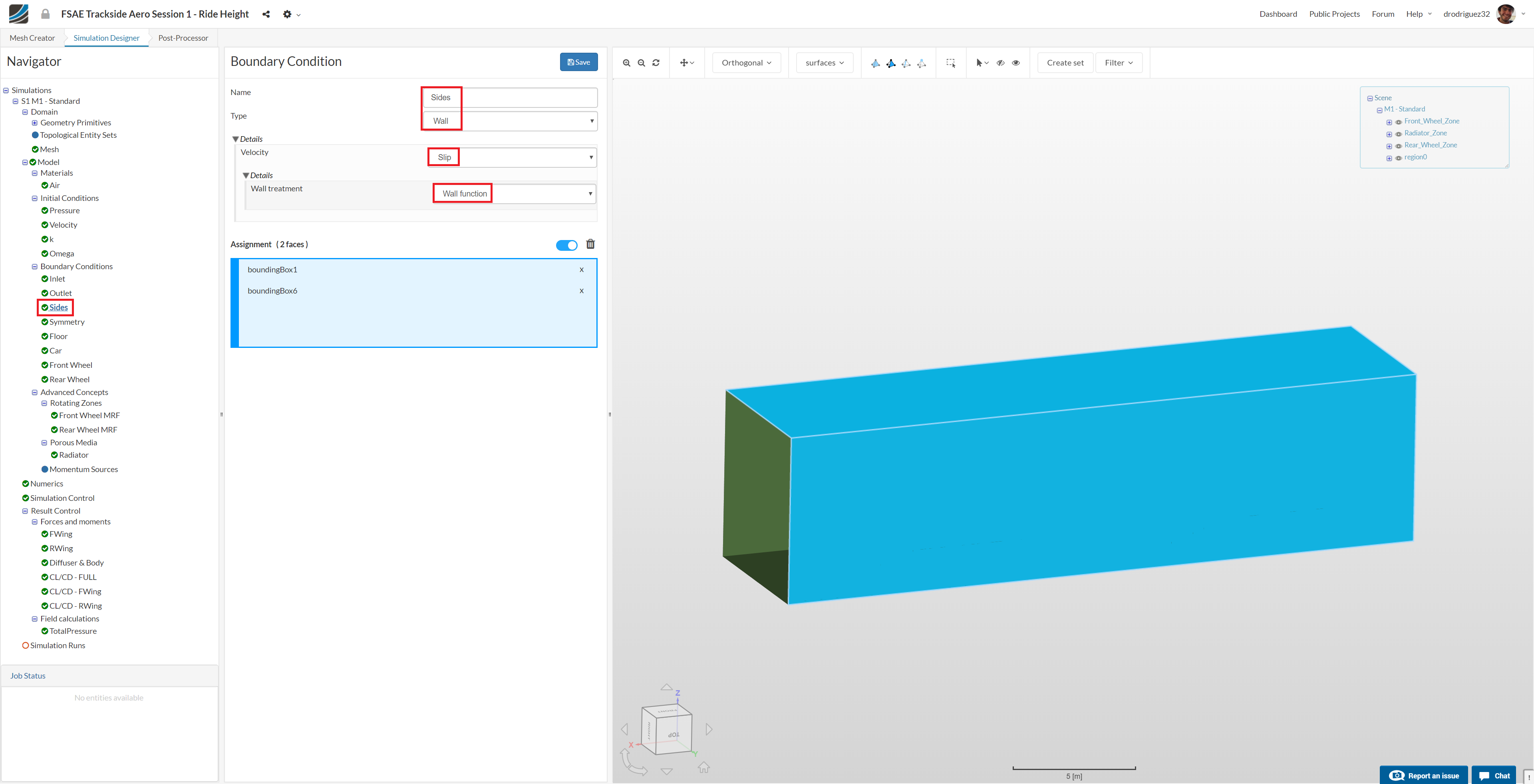
Create a new Boundary Condition and rename it to Sides (optional).
Change Type to Wall and Velocity to Slip.
Select boundingBox1 and boundingBox6 and click Save to define the boundary condition for the sides.
Remember to make sure the faces appear in the blue highlighted area titled Assignment.
Symmetry

Create a new Boundary Condition and rename it to Symmetry (optional).
Change the Type to Symmetry
Select boundingBox2 and click Save to define the symmetry boundary condition.
Floor
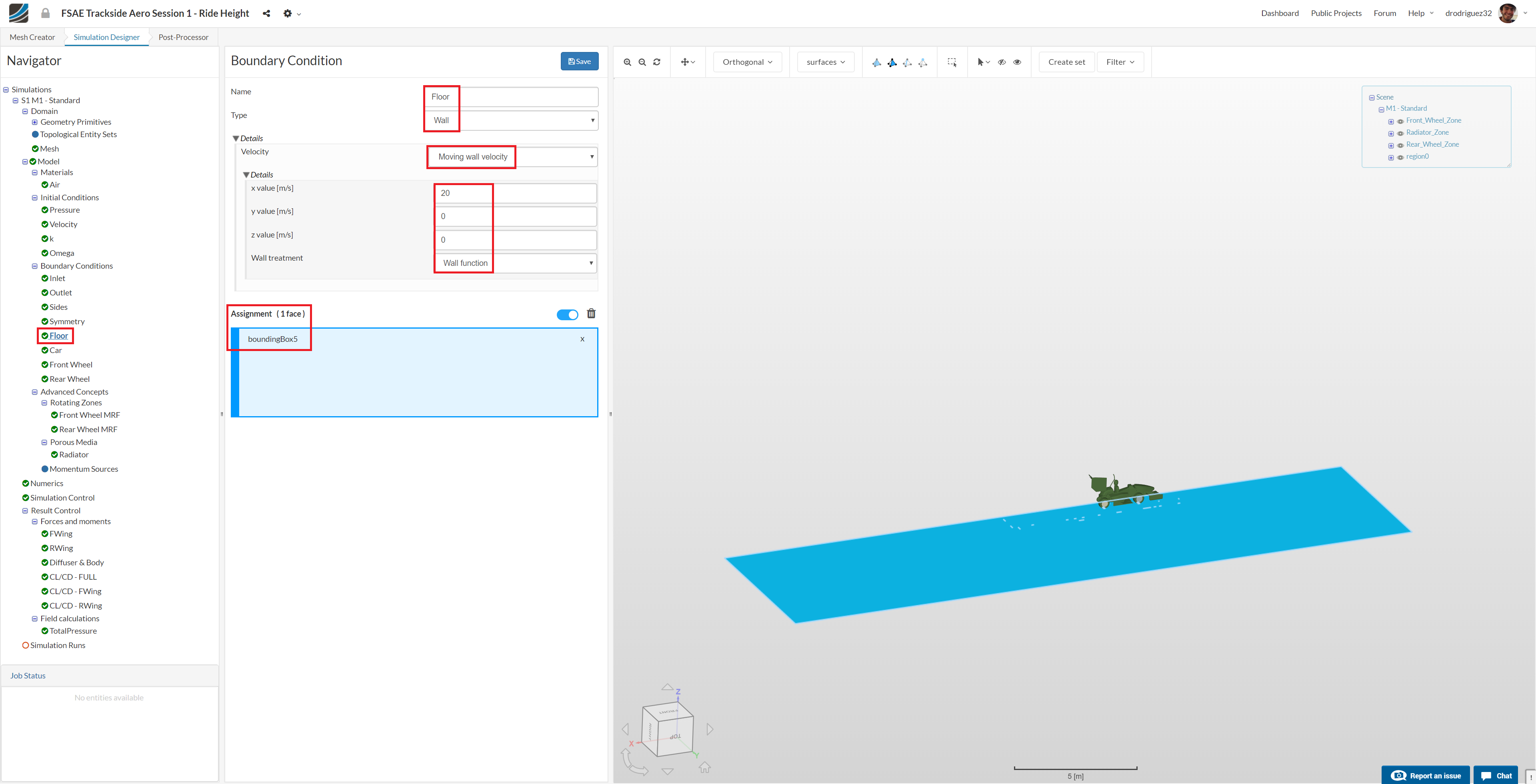
We will now define a moving floor boundary condition. Create a new boundary condition and rename it to Floor (optional).
Change Type to Wall, Velocity to Moving wall velocity and change x value [m/s] to 20
Select boundingBox5 and click Save to define the floor boundary condition.
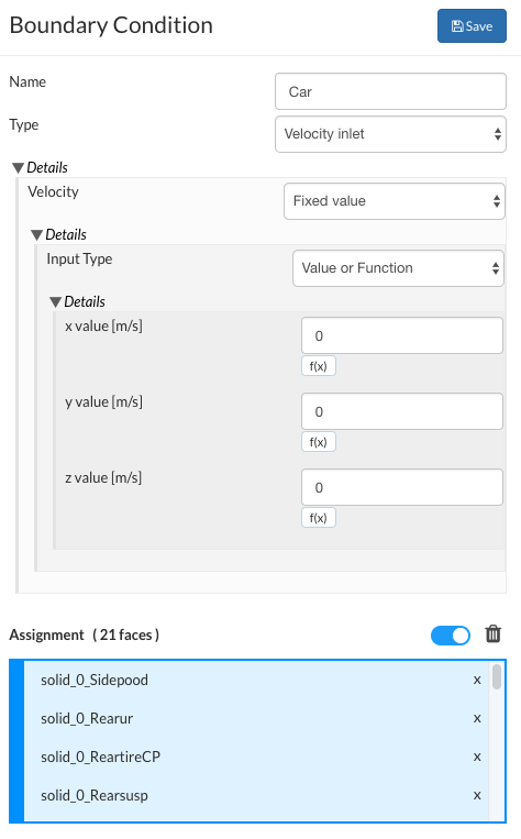
Car
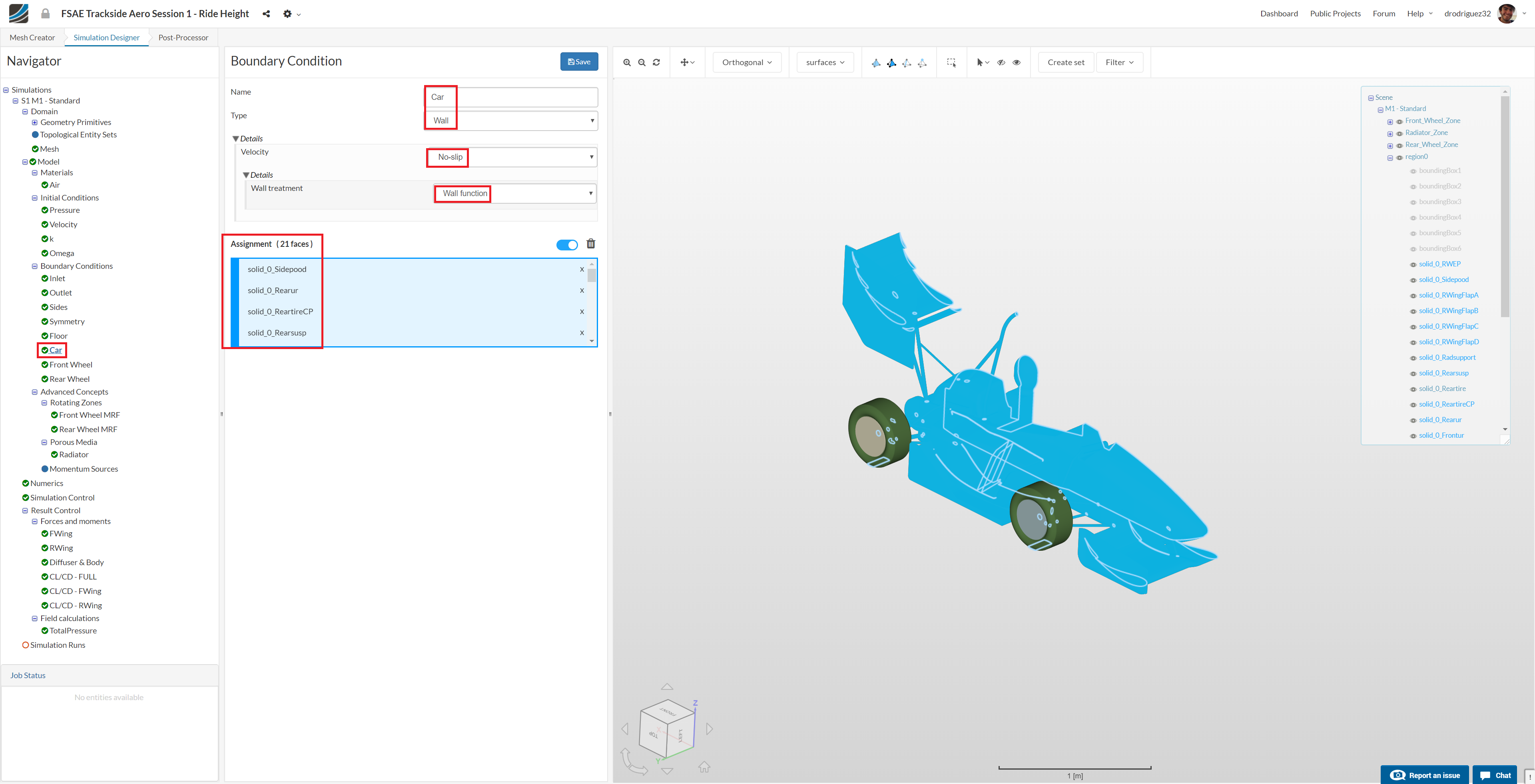
Now, we will define the boundary condition for the car. Create a new boundary condition and rename it to Car (optional).
Change the Type to Wall
Select all the entities starting with solid_0 EXCEPT solid_0_Reartire and solid_0_Fronttire from the navigator on the right.
You should have 21 faces selected.
Click Save to define the boundary condition for the car.
Rotating wheel (Front)
This is not the same thing as a Multi Reference Frame (MRF) zone.

Create a new boundary condition and rename it to Front wheel (optional).
Change the Type to Wall and Velocity to Rotating wall velocity. Then change:
- Origin x value [m], y value [m] and z value [m] value to -0.4157, 0.6 and 0.22 respectively.
- Axis of rotation x value [m] and y value [m] to 0 and 1 respectively.
- Angular velocity [rad/s] to -90.9
- Then select solid_0_Fronttire.
- Click Save to register your changes.
Make sure your setup looks like the picture above.
Rotating wheel (Rear)
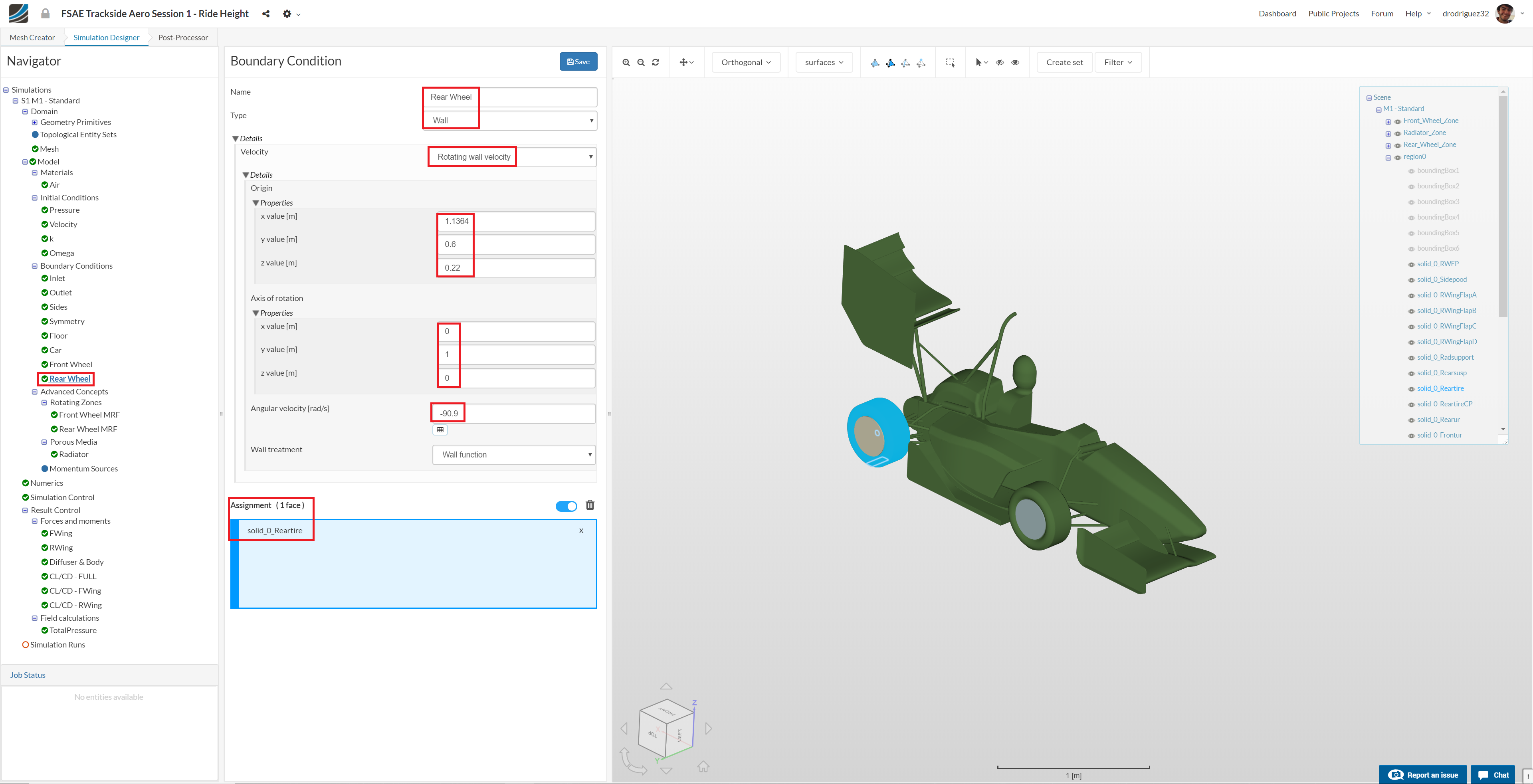
Duplicate the previous boundary condition by right clicking on it and selecting Duplicate. Rename it to Rear wheel (optional).
Change the Type to Wall and Velocity to Rotating wall velocity. Then change:
- Origin x value [m], y value [m] and z value [m] value to 1.1364, 0.67 and 0.22 respectively.
a. Notice that the origin values for the y axis and z axis are the same as the previous boundary condition. That’s why it was better to duplicate it. - Axis of rotation x value [m] and y value [m] to 0 and 1 respectively.
- Angular velocity [rad/s] to -90.9
- Then select solid_0_Reartire.
- Click Save to register your changes.
Rotating Zones (MRF)
Now we will finally create the MRF zones for the wheel rims.
Go to Advanced Concepts and click on Rotating Zones in the navigator on the left. Then click on New to setup a new rotating zone.
MRF Front

Now rename it to MRF Front
Then change:
-
Origin x value [m], y value [m] and z value [m] value to -0.4157, 0.6 and 0.22 respectively.
-
Axis of rotation y value [m] to 1
-
Angular velocity [rad/s] to -90.9
-
Then select FrontWheelZone. You should see it in the blue highlighted box under MRF zones and highlighted in blue in the viewer.
-
Make sure your settings match the picture and then click Save to register your changes.
MRF Rear
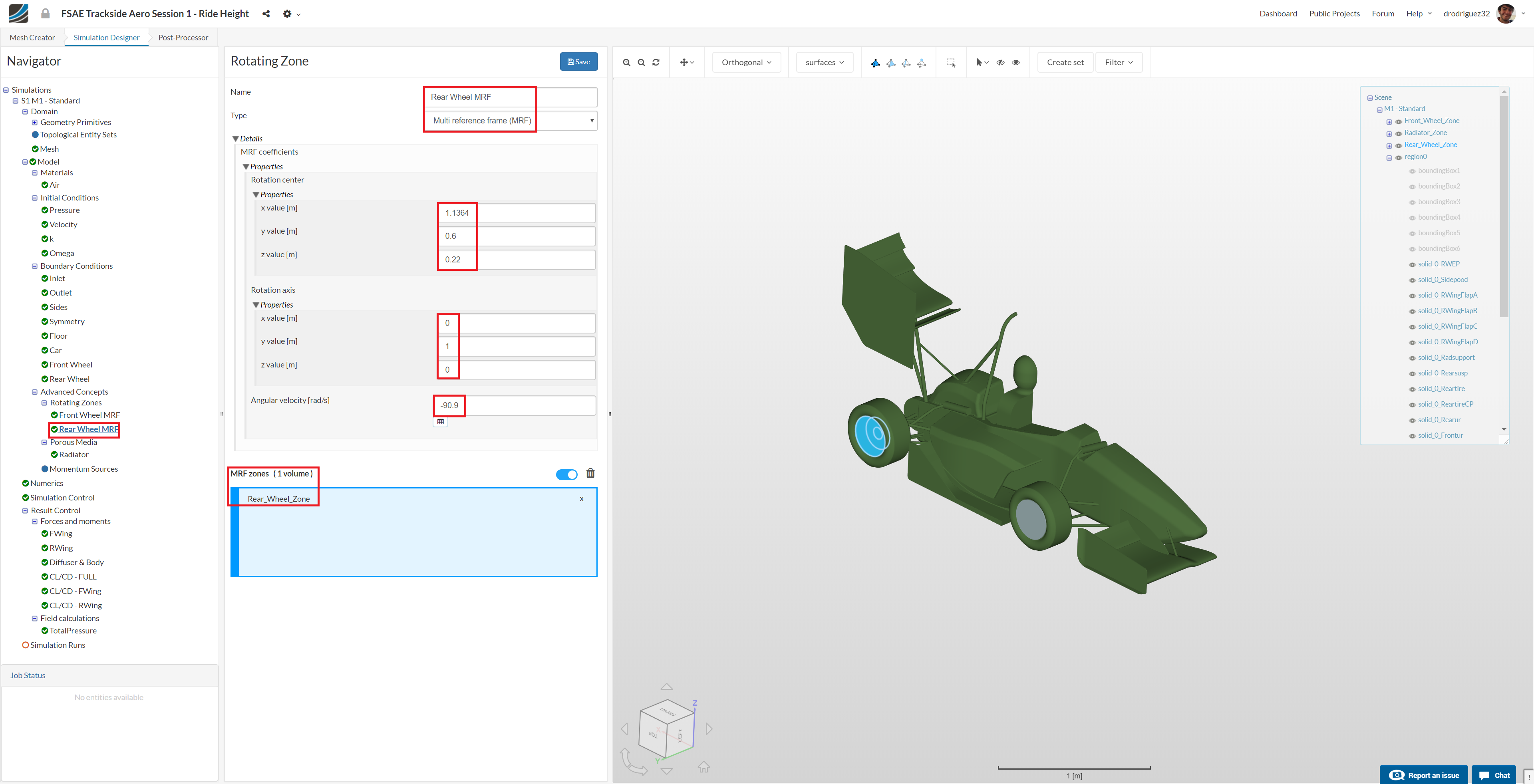
Similarly, perform the same procedure and create a new Rotating Zone. Rename it to MRF Rear. Then change:
-
Rotation center x value [m], y value [m] and z value [m] value to 1.1364, 0.6 and 0.22 respectively.
a. Notice that the values for the y axis and z axis are the same as for the front wheel -
Rotation axis y value [m] to 1.
-
Angular velocity [rad/s] to -90.9
-
Then select RearWheelZone. You should see it in the blue highlighted box under MRF zones and highlighted in blue in the viewer.
-
Click Save to register your changes.
Porous Media
Radiator
Expand the Advanced Concepts tree item and proceed to Porous Media. Click +New to create a new porous media definition.

After creating a new porous media definition, you will be automatically directed to the its properties panel. Now that you know how porous media works you can apply it to your own designs. For the sake of simplicity, we have made an approximation of the coefficients of this radiator to make it simpler and more straight forward. The vector is the correct calculated normal for the local flow direction. Change:
-
Name to Radiator - Porous Media (optional) and set the Type to Darcy-Forchheimer
a. This Darcy-Forchheimer is the model that will be used. The Darcy part states that the flow through the porous medium is proportional to the pressure drop. The Forchhiemer part is a nonlinear term for flows with high reynolds numbers that takes into account the inertial effects. -
Coefficient d x, y and z values to 20,000,000, 0, and 0 respectively.
a. This is the Darcy coefficient, or the linear part of the model. -
Coefficient f x, y and z values to 2000, 0, and 0 respectively.
a. This is the Forchheimer coefficient. -
Coordinate system e1 x, y and z values to 0.93, 0.15 and 0.34 respectively.
a. This is the vector that tells the model the local flow direction. -
Coordinate system e3 x, y and z values to -0.34, -0.054 and 0.94 respectively.
a. This is a vector that is orthogonal to e1. -
Scroll down and select RadiatorZone from the navigator on the right. Make sure it appears in the blue box under Assignment.
-
Click Save to register your changes.
Numerics
After defining all the boundary conditions, we will proceed to set up the numerics for our simulation.
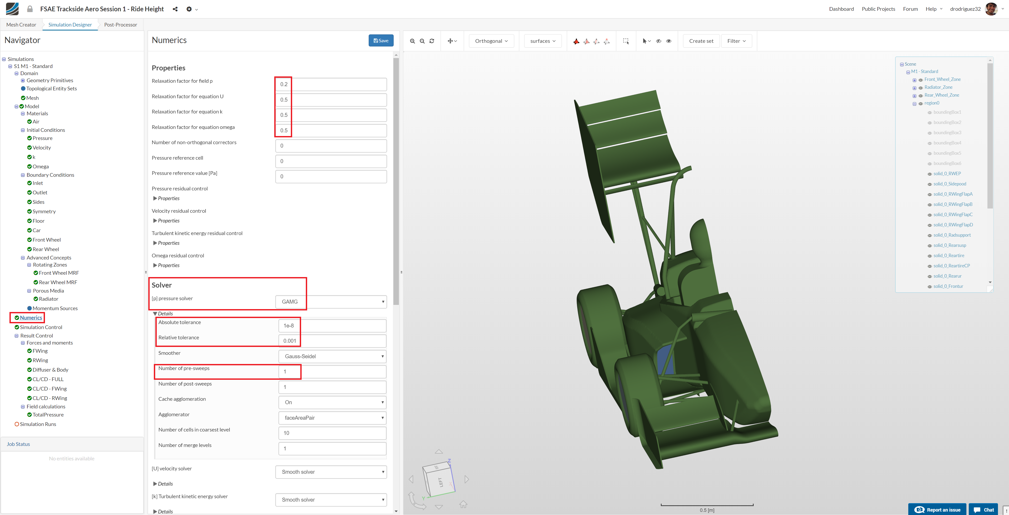
Go to Numerics and change:
-
Relaxation factor for field p, Relaxation factor for equation U, Relaxation factor for equation k and Relaxation factor for equation omega to 0.2, 0.5, 0.5 and 0.5 respectively.
-
Furthermore, under [p] pressure solver, change Absolute tolerance, Relative tolerance and Number of pre-sweeps to 1e-8, 0.01 and 1 respectively.
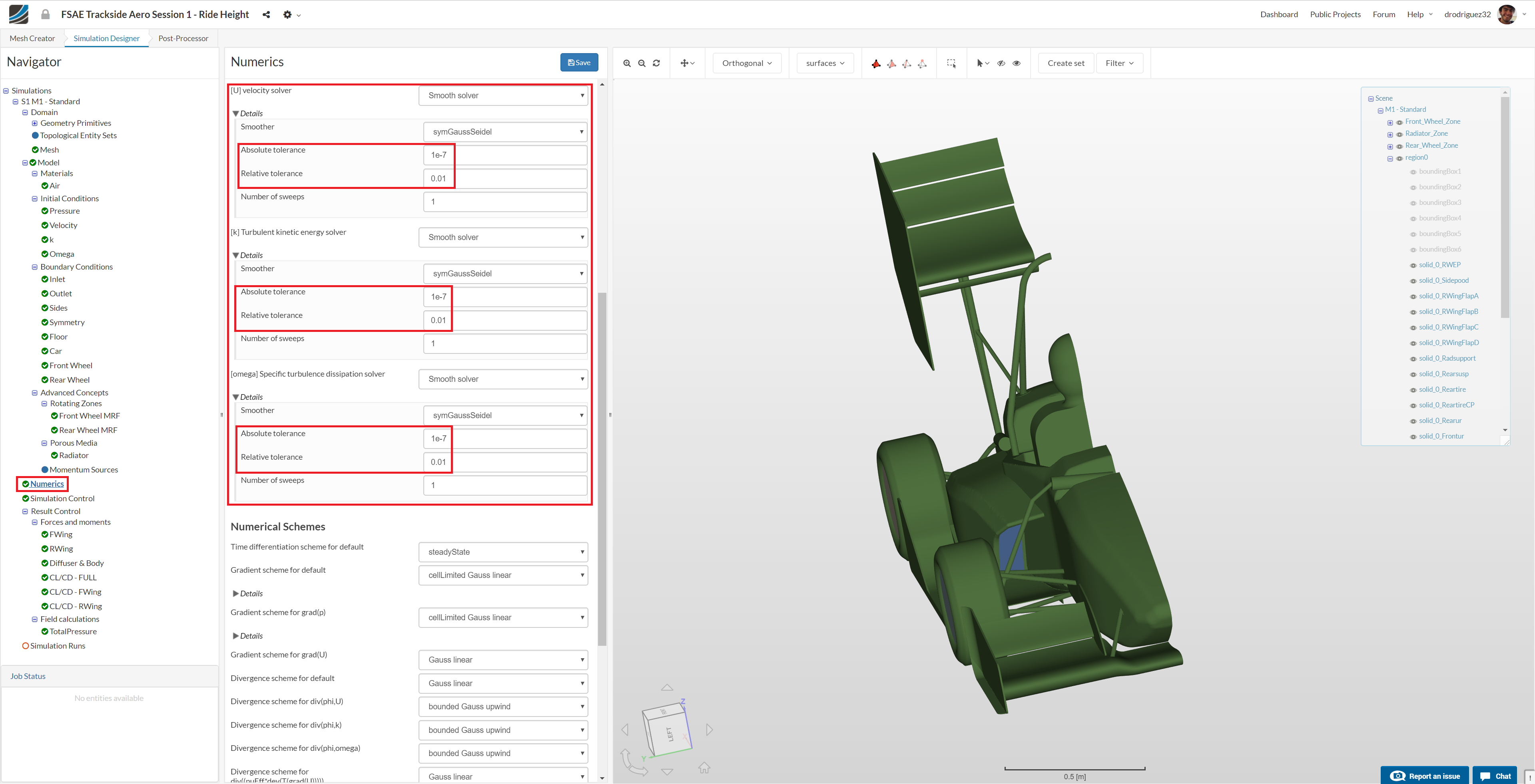
Scroll down until [U] velocity solver and change:
- [U] velocity solver to Smooth solver, Smoother to symGaussSeidel and Absolute tolerance to 1e-7.
Do the same for [k] Turbulent kinetic energy solver and [omega] Specific turbulence dissipation solver.

Change both Gradient scheme for default and Gradient scheme for grad p to cellLimited Gauss linear
Scroll down to the end and change:
-
Laplacian scheme for default, Laplacian scheme for laplacian(nu,U), Laplacian scheme for laplacian(nuEff,U) and Laplacian scheme for laplacian((1|A(U)),p) to Gauss linear limited corrected
-
Click Save to register all of your changes.
Simulation Control
Next we will define our simulation interval and steps that needs to be recorded.
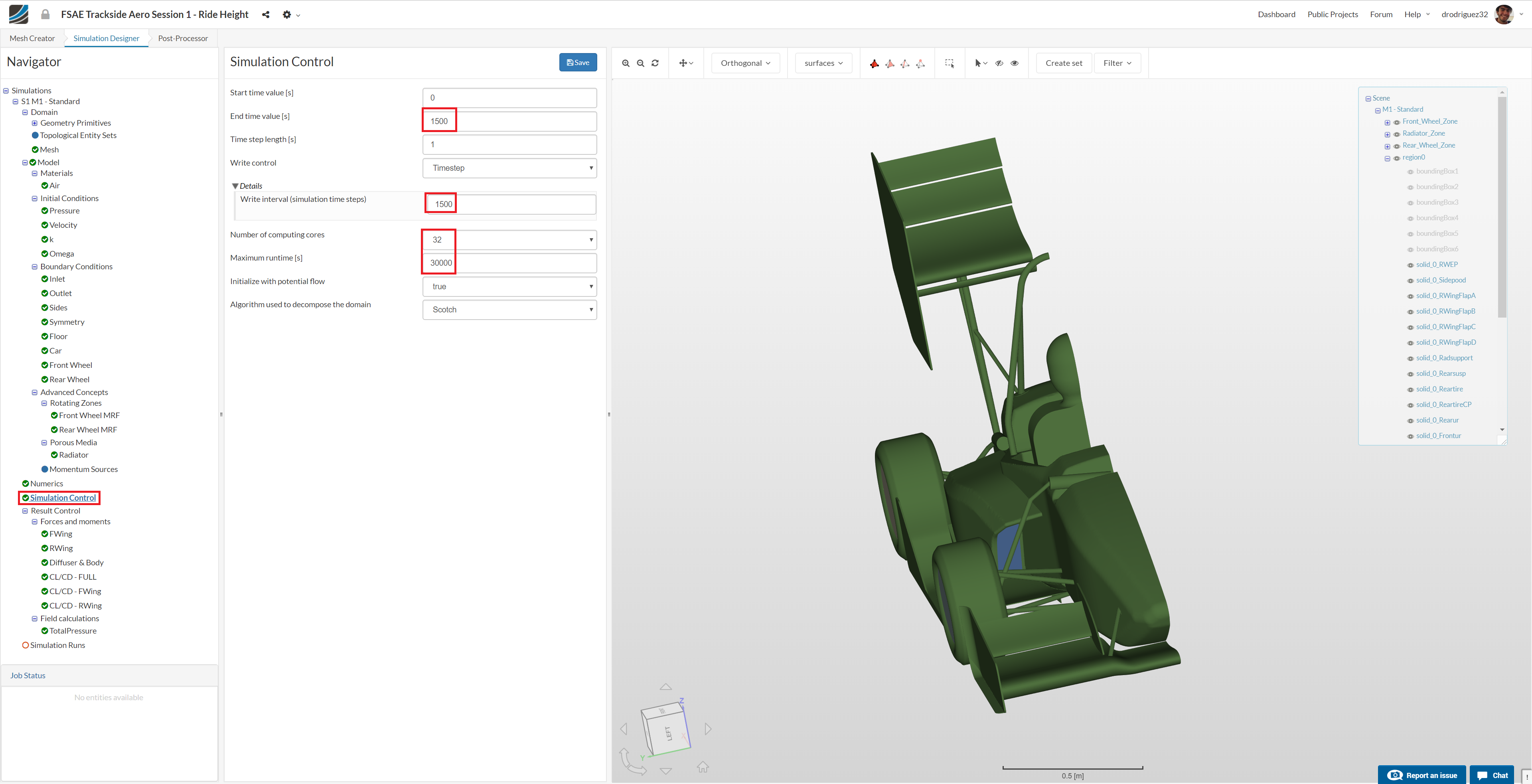
Go to Simulation Control and change End time value [s] to 1500.
Expand Details under Write control and change Write interval (simulation time steps) to 1500.
Next change Number of computing cores and Maximum runtime [s] to 32 and 30000 respectively.
Click Save to register your changes.
Result Control
As our last step before running the simulation, we will create result control items in order to get graphical data sets of interest.
Firstly, we will create the result control item for the forces and moments. Go to Result Control and click New next to Forces and Moments.
A new force and moment result control item will be created.
Front Wing
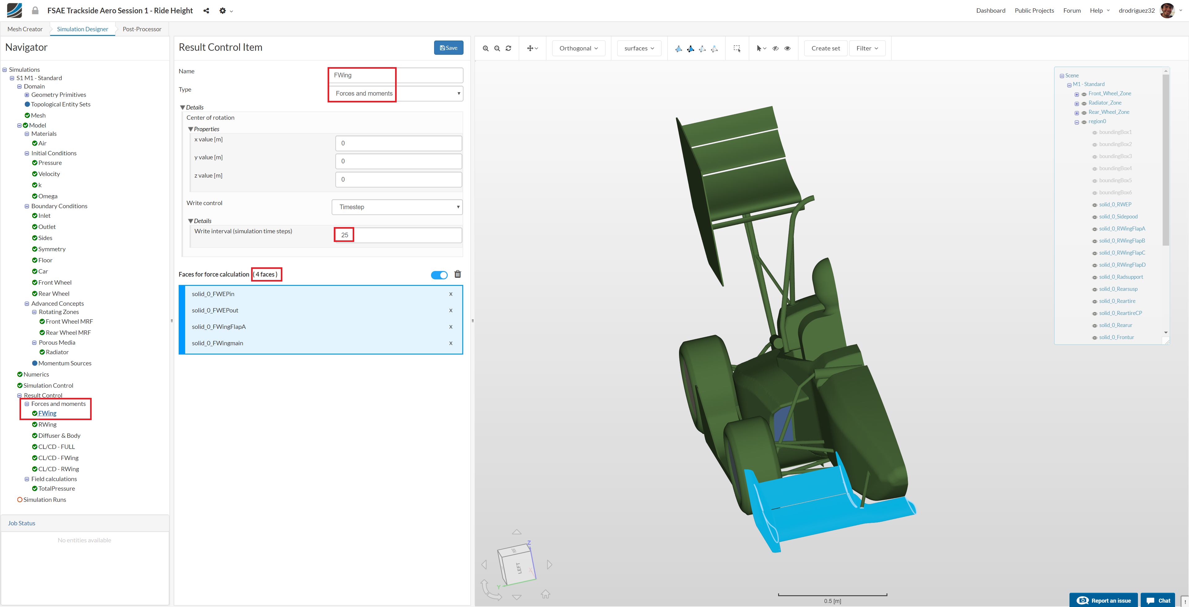
Rename it to FWing (optional).
Then change Write interval (simulation time steps) 25.
Select solid_0_FWmainwing, solid_0_FWEPin, solid_0_FWEPout and solid_0_FWflap. You should see them under Faces for force calculation.
Click Save to register your changes.
Rear Wing

Create another force and moment result control item and rename it to RWing (optional).
Then change Write interval (simulation time steps) 25.
Select solid_0_RWEP, solid_0_RWflapa, solid_0_RWflapb, solid_0_RWflapc and solid_0_RWflapd. You should see them under Faces for force calculation.
Click Save to register your changes.
Diffuser & Body

Follow the same procedure to create force and moment result control item for the diffuser. Rename it to Diffuser & Body (optional).
Then change Write interval (simulation time steps) 25.
Select solid_0_Diffuser, and solid_0_Body.
Click Save to register your changes.
Lift & Drag Coefficients
In order to do our Aero Map, we need to calculate the lift and drag coefficient for the car.
In order to do this, create a new Result Control Item under Forces and Moments, but under the drop down menu select Forces and Moments Coefficients.
Full Car
Create the result control item and rename it to “CL/CD - FULL” (Optional).

Make the lift direction (0,0,1)
Make the drag direction (1,0,0)
Make the pitch axis (0,1,0)
Change the Freestream Velocity to 20
The next two values (length and area) will influence the calculation of these coefficients. So depending on the model you’re working on (for this tutorial it’s the Standard), use the following table to define area and length
| Model Name | Length [m] | Area [m^2] |
|---|---|---|
| Standard | 3.08 | 0.5441 |
| Low Nose | 3.07 | 0.5478 |
| Low Nose 2 | 3.06 | 0.5534 |
| Low Rear | 3.09 | 0.5424 |
| Low Rear 2 | 3.10 | 0.5417 |

Change the Write Interval to 25.
Select ALL the faces that start with solid_0, and also select the Radiator_Zone.
You should have 24 faces selected.
Front Wing
Create the result control item and rename it to “CL/CD - FWing” (Optional).

Make the lift direction (0,0,1)
Make the drag direction (1,0,0)
Make the pitch axis (0,1,0)
Change the Freestream Velocity to 20
The next two values (length and area) will influence the calculation of these coefficients. So depending on the model you’re working on (for this tutorial it’s the Standard), use the following table to define area and length
| Model Name | Length [m] | Area [m^2] |
|---|---|---|
| Standard | 0.64 | 0.3664 |
| Low Nose | 0.64 | 0.3659 |
| Low Nose 2 | 0.64 | 0.3657 |
| Low Rear | 0.64 | 0.3667 |
| Low Rear 2 | 0.64 | 0.3671 |
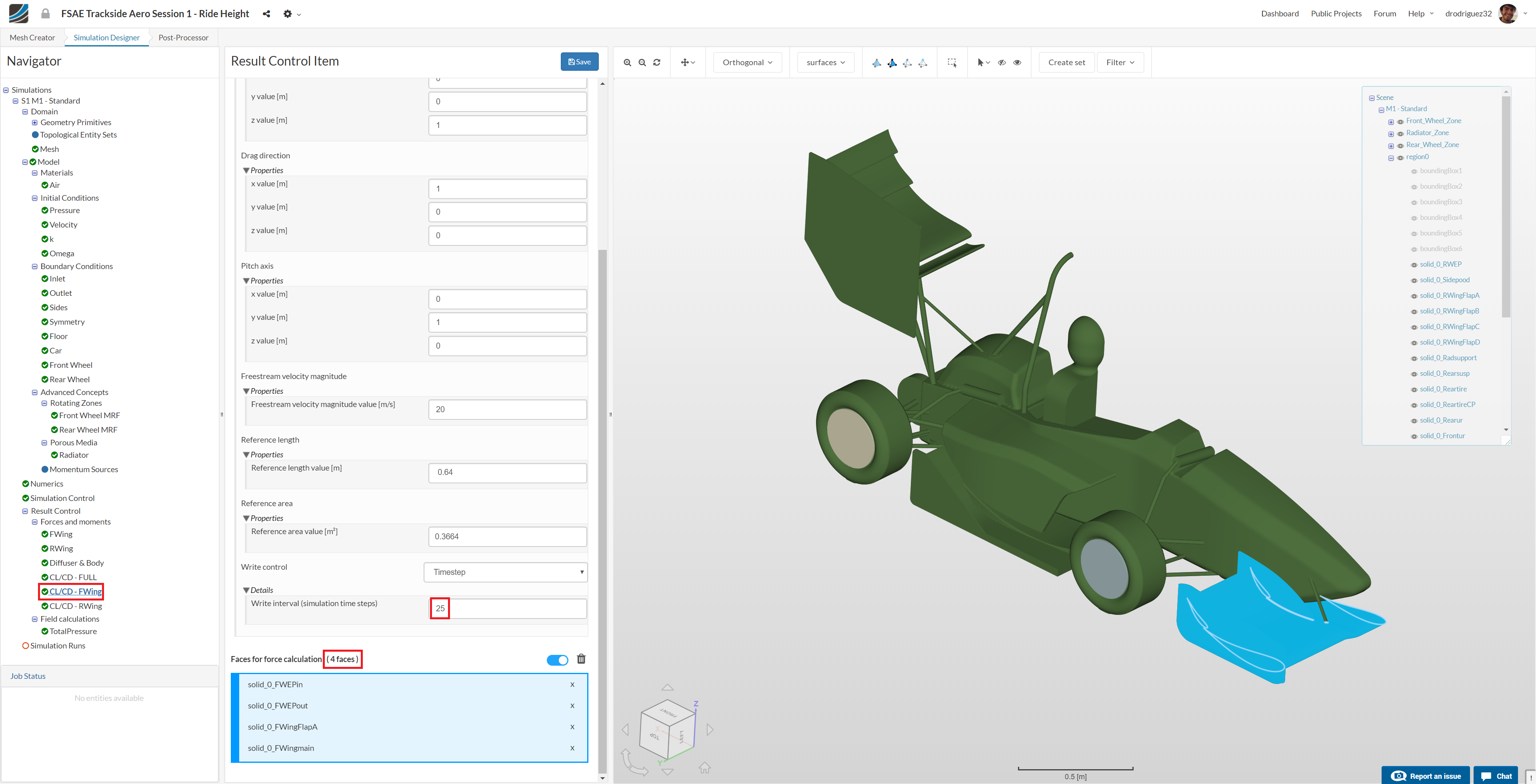
Change the Write Interval to 25.
Select the elements for the front wing.
You should have 4 faces selected.
Rear Wing
Create the result control item and rename it to “CL/CD - FWing” (Optional).
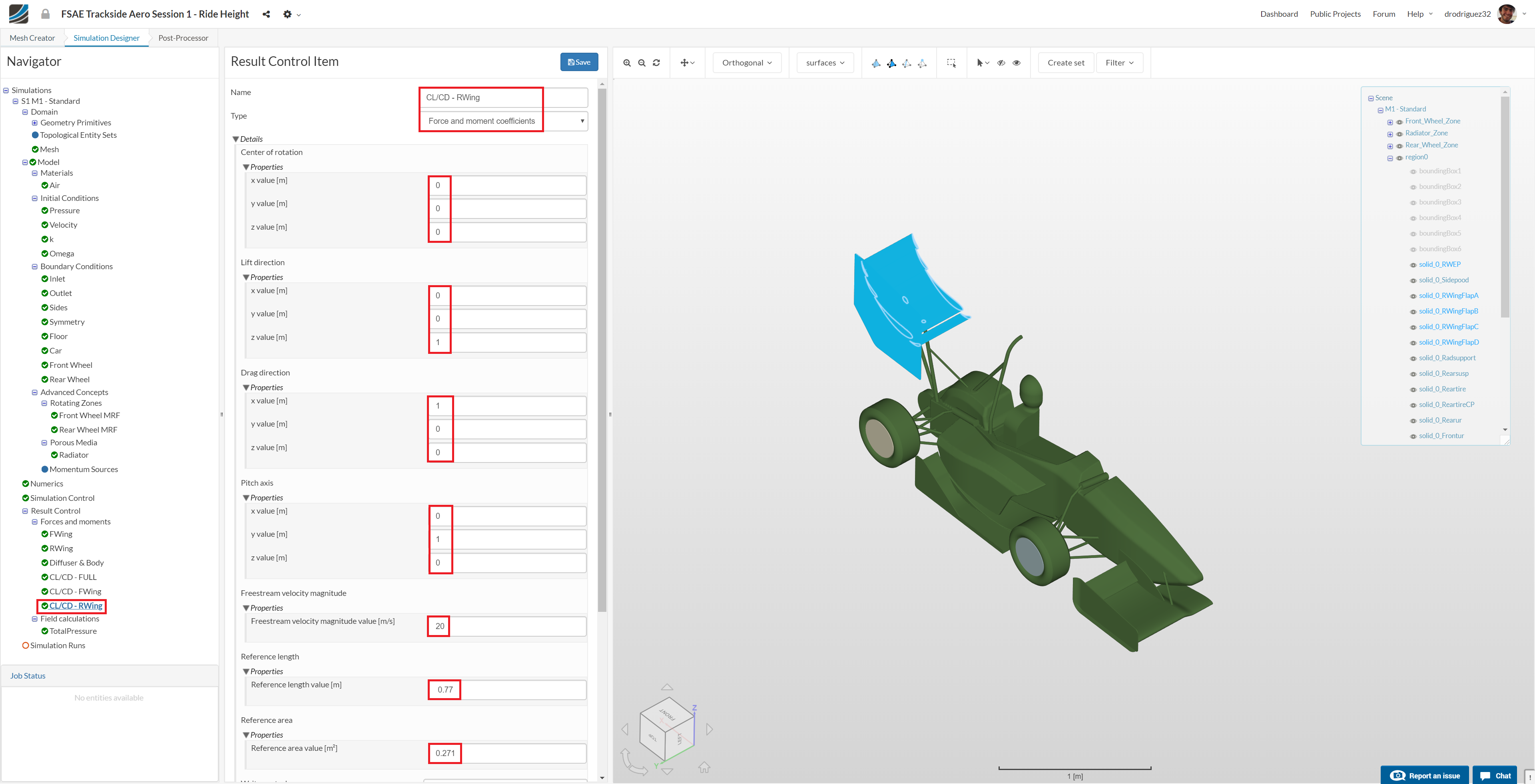
Make the lift direction (0,0,1)
Make the drag direction (1,0,0)
Make the pitch axis (0,1,0)
Change the Freestream Velocity to 20
The next two values (length and area) will influence the calculation of these coefficients. So depending on the model you’re working on (for this tutorial it’s the Standard), use the following table to define area and length
| Model Name | Length [m] | Area [m^2] |
|---|---|---|
| Standard | 0.77 | 0.2710 |
| Low Nose | 0.77 | 0.2694 |
| Low Nose 2 | 0.77 | 0.2680 |
| Low Rear | 0.77 | 0.2717 |
| Low Rear 2 | 0.77 | 0.2732 |
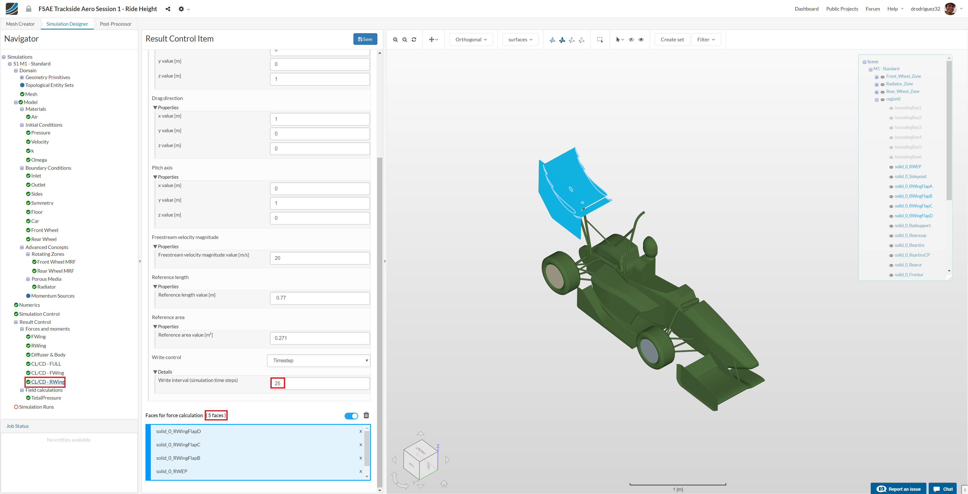
Change the Write Interval to 25.
Select the elements for the rear wing.
You should have 5 faces selected.
Simulation Run

Once all the above steps are defined, we will proceed to create our first simulation run. Go to Simulation Runs and click on New and then Create in order to create a new run.
After the run is created, click Start to start the created run. The simulation run can take up to ~230 minutes (~5 hrs.)
Since you have just run the simulation for the Standard model, we have provided you the results for the low nose and low rear conditions at the link below:
Post-Processing
When your simulation is finished and you go to the Force Coefficient Plots in the Post-Processor, please just look at the ones called Lift Coefficient and Drag Coefficient. These are the C_L and C_D we’ve been taking about in the tutorial and the ones we’re interested in.
In the following comparisons, you will be able to see side by side the results for different simulations. On the top you will always have the standard setup and on the bottom you will have the varying ride heights. Take a special look at the areas where the two big black arrows in the following picture are pointing.
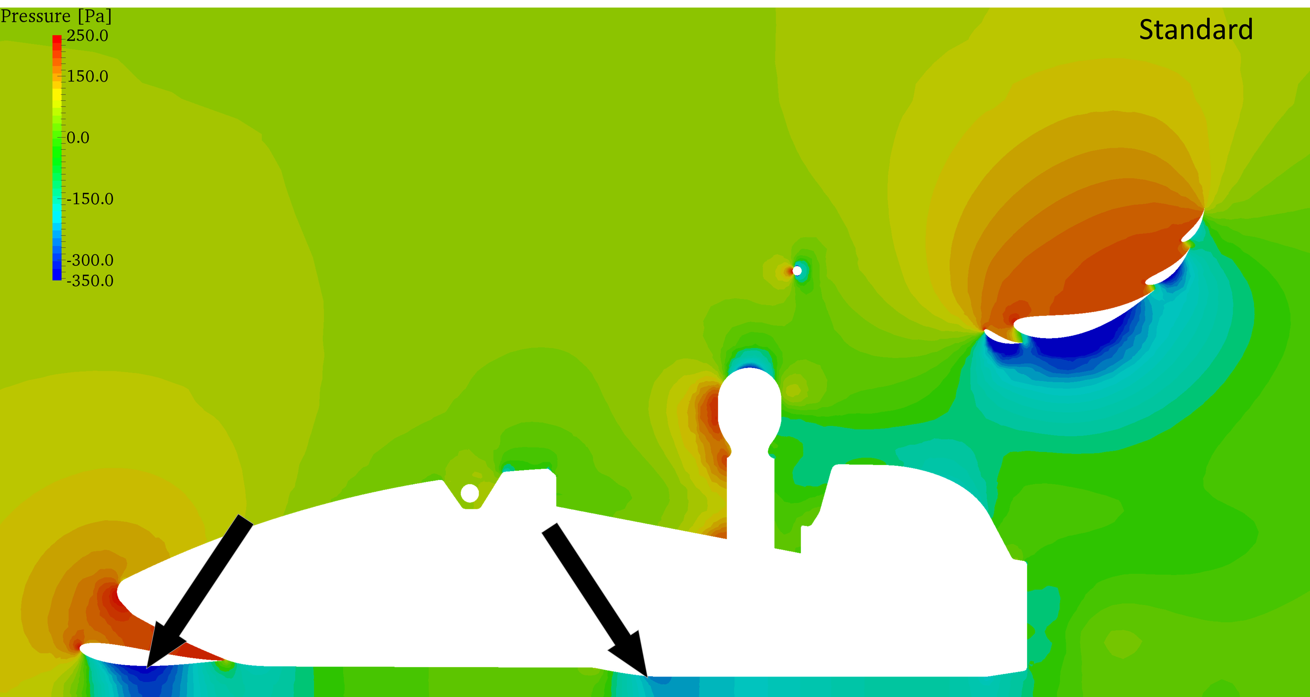
Pressure
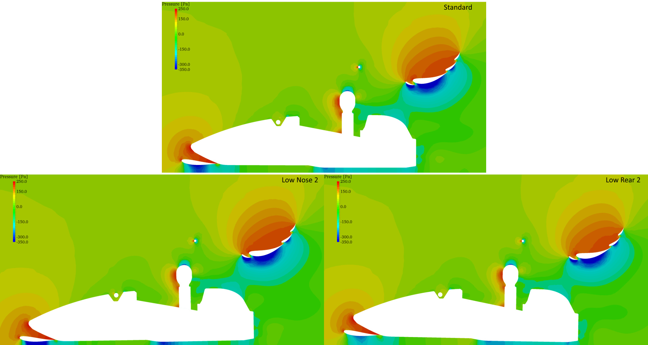
Notice how in the areas of interest there is a much bigger negative pressure area for the Low Nose setup. While the Low Rear setup loses these low pressure zones and the front wing becomes less effective - losing downforce.
Velocity
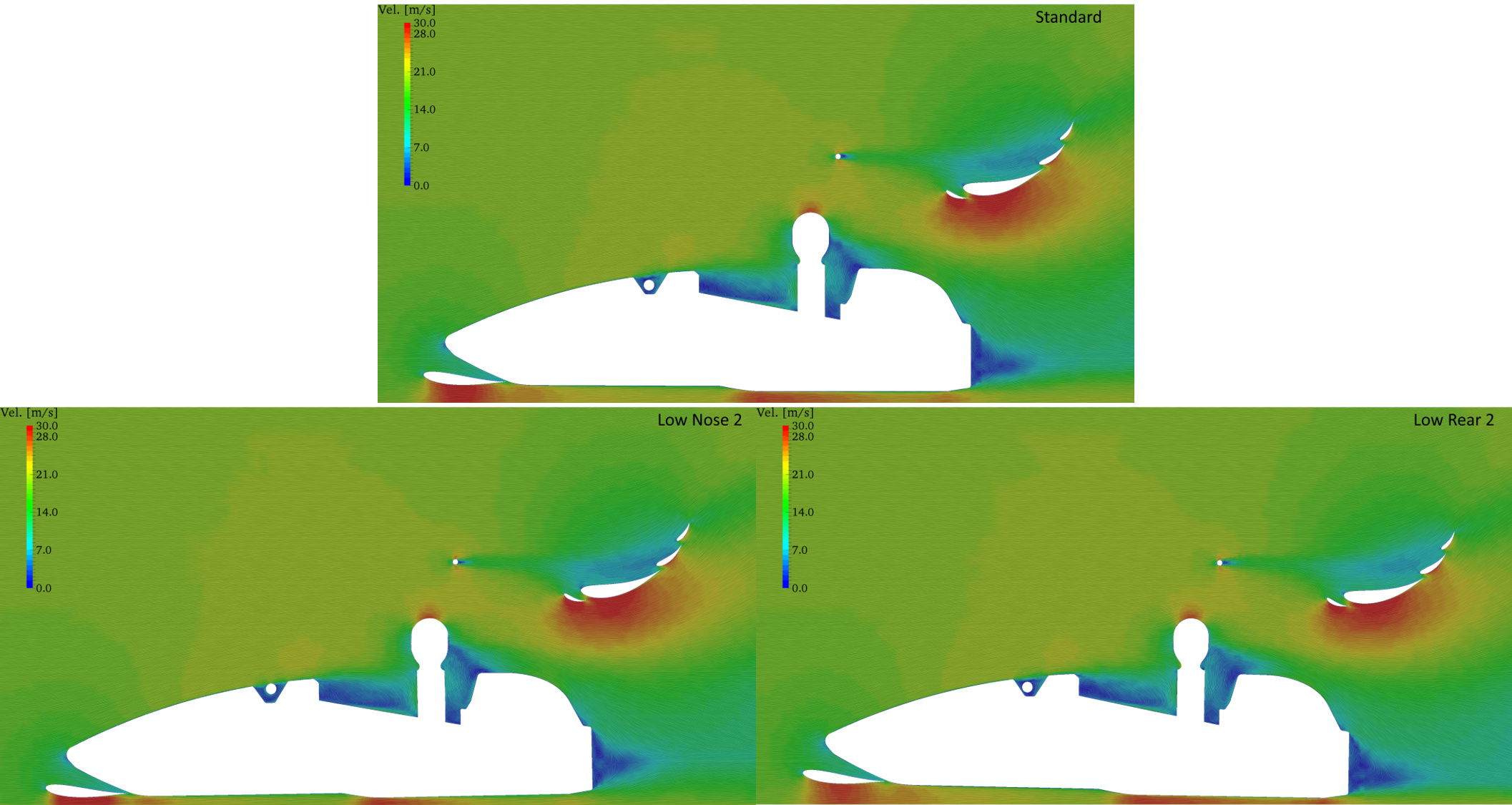
For the velocity, notice that in those areas of interest you get higher velocities as you bring the car close to the floor. This is particularly helpful for the front wing - as it comes closer to the floor the ground effect becomes more prominent and generates more downforce. Notice that when you raise the rear you lose this high velocity area at the front wing and thus make it less efficient and effective.

 thank you!
