How Do Wings Work?

jousefm · November 12, 2018, 2:13pm

\text{It is easy to explain how a rocket works, but explaining how a wing works takes a rocket scientist. } \\ \text{–Philippe Spalart}

\underline{\textbf{Table of contents}}

Motivation
History
Popular Explanations & Reductio ad Absurdum
3.1 Equal Transit Time Theory
3.2 Newton’s 3rd Law & Particle Kinetic Theory
3.3 Streamtube Pinching aka. Venturi Theory
Popular Good Explanations
4.1 Flow Turning
4.1.1 Newton vs. Bernoulli
4.2 Streamline Curvature and Mathematical Derivation
Only Low and High-Pressure Regions

\underline{\textbf{1. Motivation}}

The well-known Navier-Stokes equations are second-order partial differential equations that describe fluid motion and are derived from very fundamental physical principles, namely Conservation Laws:

• The Conservation of Momentum
• The Conservation of Mass
• The Conservation of Energy

These three principles allow the usage of the ever so famous and previously mentioned Navier-Stokes equations (NSE). As of today, the Navier-Stokes equations can accurately predict lift and are the go-to mathematical theory. However, in practice, especially in terms of using computational fluid dynamics (CFD) to predict lift, there is a need to resolve the inherent turbulence of air at the areas near the surface of the wing (also known as the Boundary Layer). Solving these is theoretically possible but highly impractical as there would be an exponential amount of resolving to do in order to predict all turbulences at this level. Not only would copious amounts of computing power be needed to resolve this area, but it may also only resolve a small area and should the conditions or model change, a complete rework would be needed.

Thus there is a need for simplification of the Navier-Stokes equations in order to have practical methods to predict lift in a relatively low-cost and timely manner. Reynolds-averaged Navier-Stokes (RANS) equations are one such method where turbulence at the Boundary Layer is averaged over time, reducing the need to solve every single one of them for the entire simulation time. Of course, there is a catch: the results will be slightly inaccurate (typically a few percents off the actual amount). Despite being slightly inaccurate, the time and computational effort saved is orders of magnitude versus directly resolving using the Navier-Stokes equations. With additions like turbulence modeling—which allows better representation of the effects at the Boundary Layer—RANS equations are popular and commonly used.

The problem with non-engineers, however, is that these equations are not very much appreciated, as they seem not very intuitive compared to Bernoulli’s equation. Especially non-engineers are interested in how big aircraft are able to fly and how lift affects other sectors like F1 cars, ship propellers or boats, and how a wing exactly produces this lift—engineers usually have to provide an answer that is intuitive as well as easy from a physical perspective. Unfortunately, the most common explanations of lift are wrong, which is not only confusing for a lot of people but can lead to a poor understanding of important aerodynamic principles. In this article, we will take the most common misconceptions and explain why they are wrong. In the end, we will give an explanation of how wings really work along with a mathematical derivation that you can easily memorize.

Before delving further into the theory, it is important to know a bit more about wings and in particular, the first thing that comes to mind when you ask an engineer what a wing is: an aerofoil. An aerofoil is the shape of the wing, typically seen by its cross-section. The shape, length, camber, thickness, and position of the aerofoil all affect the performance of the wing adversely. Optimizing these parameters for a particular use case is typically the result of thousands of talented engineers working years to develop the perfect aerofoil and wing for their area of application. For our purposes, we will be strictly referring to a simple 2D aerofoil. It is also important to note that the most important force is lift.

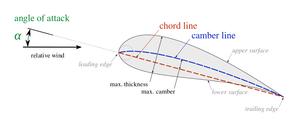
Figure 1: Airfoil nomenclature

Please keep in mind that the mechanisms and underlying theories that allow such a fundamental device to work can be difficult to understand and intimidating at first glance. While this article will not make you an expert in wings, it will give you some insight into how they work and as previously mentioned, teach you common misconceptions about these fascinating devices.

\underline{\textbf{2. History}}

A wing, by definition, is a type of fin that produces lift when moving through a medium such as air. According to this definition, the movement of the same fin through other mediums such as water will also generate lift. Ever since Orville and Wilbur Wright famously conceived and built the first heavier-than-air aircraft from basic materials over a 100 years ago, everyone you meet will certainly be able to tell you what a wing is.

Wings have come a very long way even when compared to 50 years ago. From the iconic bi-planes during World War 1 to the legendary World War 2 fighter aircraft, and from the Supermarine Spitfire with its highly efficient elliptical wings finally to modern wonders like the mind-bogglingly fast SR71, the evolution of wings has made aircraft faster and more efficient than ever. The underlying principles, however, remain the same.

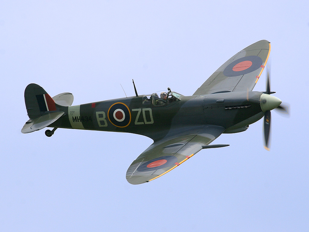
Figure 2: Supermarine Spitfire

Aerodynamics is the underlying branch for wings in flight. In the most basic terms, a wing generates a lifting force perpendicular to the direction of flow (usually and ideally forward). If the lifting force is sufficient to overcome the drag (a force parallel and opposite to the direction of flow) and weight of the object, then the object is able to fly.

\underline{\textbf{3.1 Equal Transit Time Theory}}

Figure 2 shows the cross-section of an airfoil with its pressure distribution along with the corresponding stagnation point (denoted by S) and trailing edge at the end of the airfoil (denoted by T). The common concept of the so-called “equal transit time theory” states that fluid particles that separate at the stagnation point should meet again at the trailing edge which requires that the upper fluid parcel travels faster than its counterpart on the bottom. This increase in velocity is now connected with Bernoulli’s equation (1) stating that larger velocities imply lower pressure and vice versa, resulting in a net upward pressure force that lifts the airfoil.

p + \frac{1}{2}\rho v^2 = const. \tag{1}

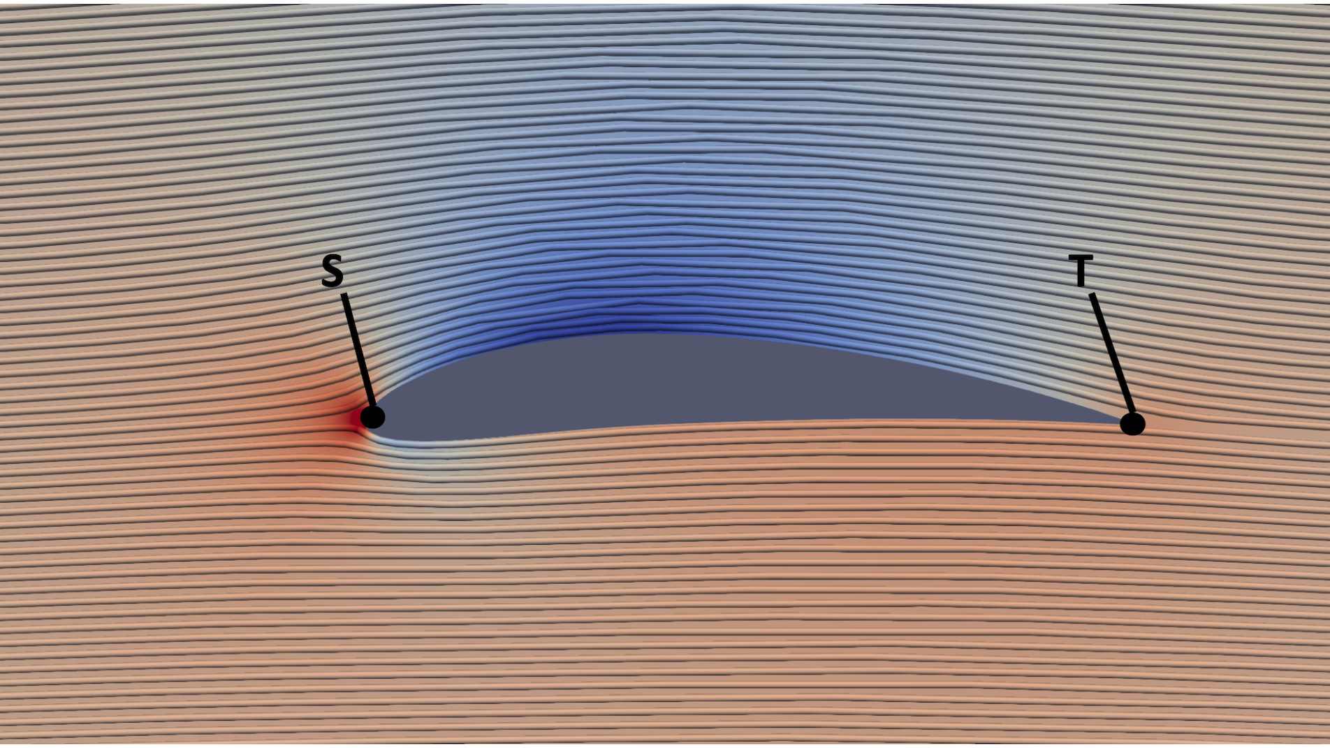
Figure 3: Pressure distribution across an airfoil

Many times, this phenomenon is demonstrated by blowing over a piece of paper as depicted in figure 3. However, there is an easy counterexample to this “experiment”. Simply blow over a paper that is hanging straight (vertically) and you will see that there is no movement. It is absolutely forbidden to make assumptions about the pressure and velocity across different streamlines! We can use Bernoulli’s equation only along a streamline.

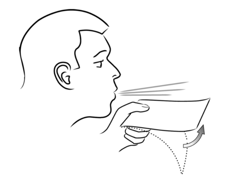
Figure 4: The “classic” experiment to demonstrate how a wing works

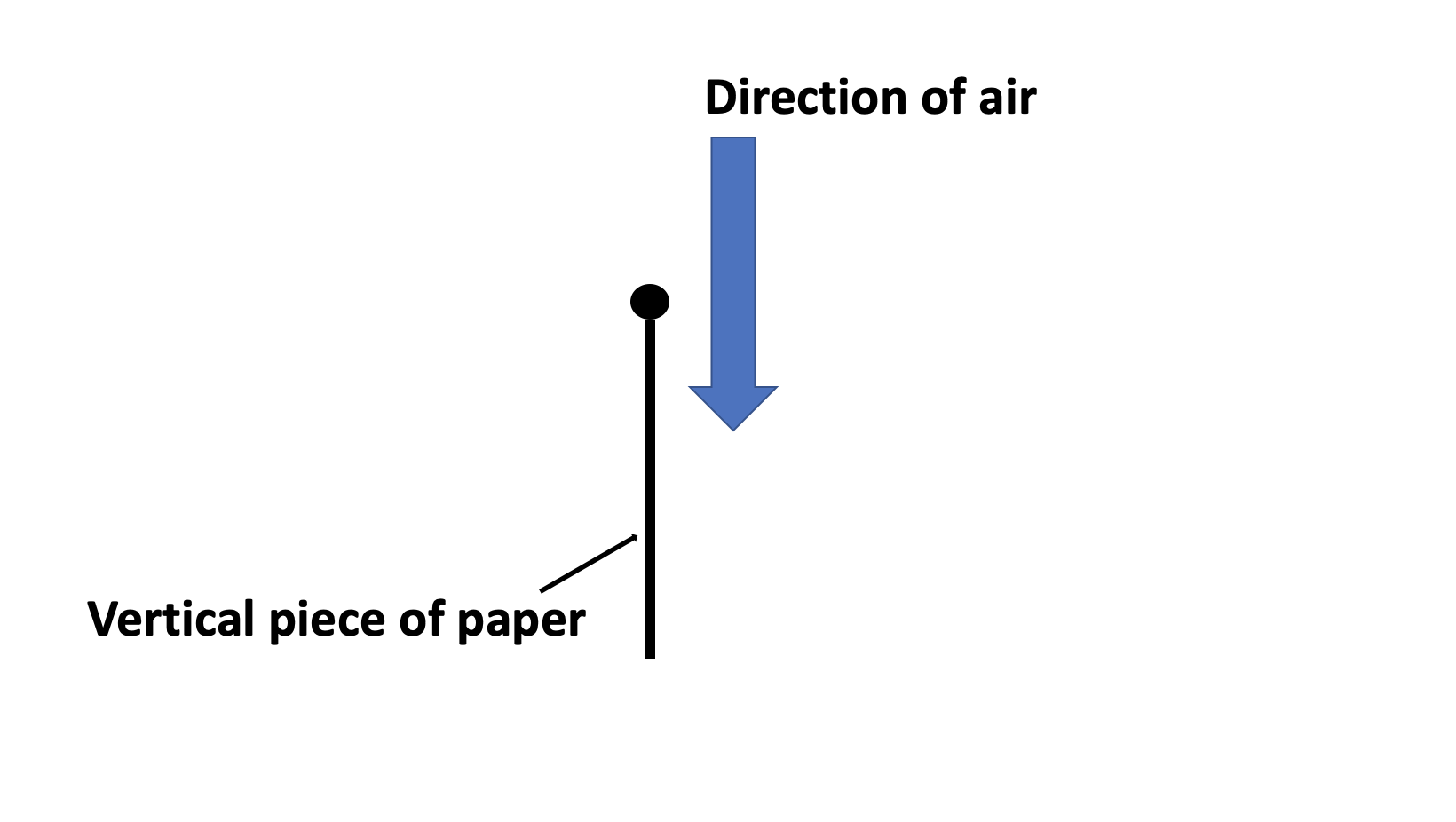
Figure 5: Counterexample for the experiment depicted in figure 4

What is also interesting in this case is that if you visualize the streamlines over an airfoil, one can conclude that the path difference highly underestimates the lift that is generated as the velocity differences are simply too small. A visualization is given in the video below where aerodynamics expert Professor Holger Babinsky from the University of Cambridge’s Department of Engineering debunks the popular, yet misleading, explanation of how wings lift.

Another thing that we have to keep in mind is that if we look at fluid parcels close to the wall or even at the wall, the transit time would tend to infinity and even at the stagnation point the same scenario would occur due to the so-called “no-slip” condition. Now we could overcome this problem by saying that we go outside the viscous boundary layer to look at fluid parcels, but still, the error is an order of magnitude, too big to explain the effect of lift.

Additional information: This theory cannot explain how aircraft can fly upside down or how a flat plate can generate lift!

\underline{\textbf{3.2 Newton's 3rd Law & Particle Kinetic Theory}}

Another widespread theory is the so-called particle kinetic theory which states that molecules are reflected downwards and—similar to the explanation of how rockets work—a reaction force must act on the airfoil pushing it up. This is simply Newton’s 3rd law, stating that for every action there is an equal and opposite reaction.

The problem with this explanation is that you only look at the molecules in front of the airfoil and those that are deflected, but neglect the ones that are behind the airfoil, making a grave assumption saying that there is no interaction between the molecules. However, this is fundamental in order to describe fluids, thus this explanation cannot be true.

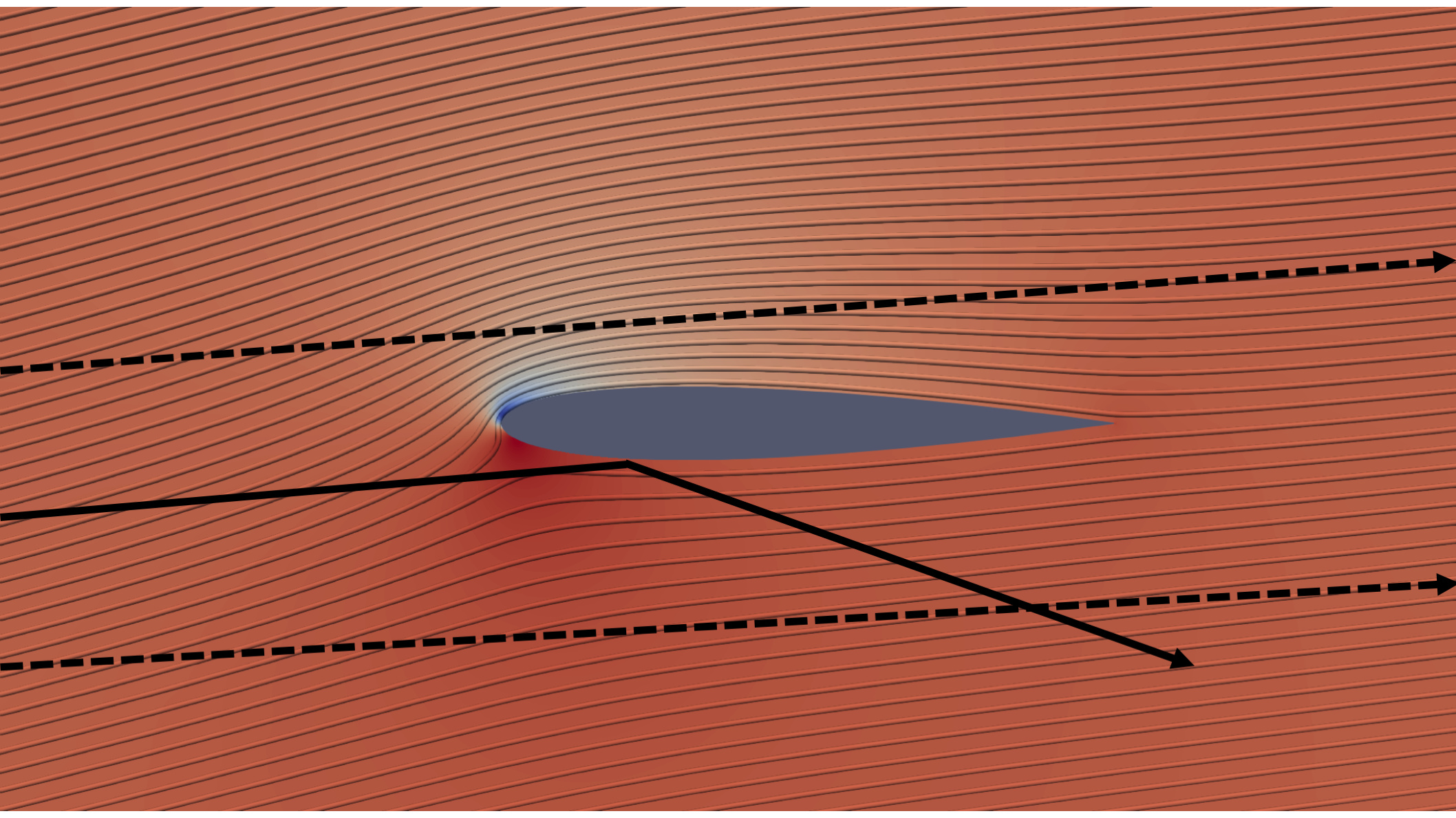
Figure 6: Visualization of incoming and deflected molecules (black lines) – Pressure distribution shown

Another argument against this theory can be proven mathematically. When looking at the lift, one finds that the lift proportional to the square of the angle of attack (AoA),

\text{lift} \propto sin^2(\alpha) \tag{2}

that uses two angles (one of the incoming stream and one for the deflected stream). But please keep in mind that the lift has a linear relation with the angle of attack,

\text{lift} \propto sin(\alpha) \tag{3}

which again shows the weakness of this erroneous theory.

\underline{\textbf{3.3 Streamtube Pinching aka. Venturi Theory}}

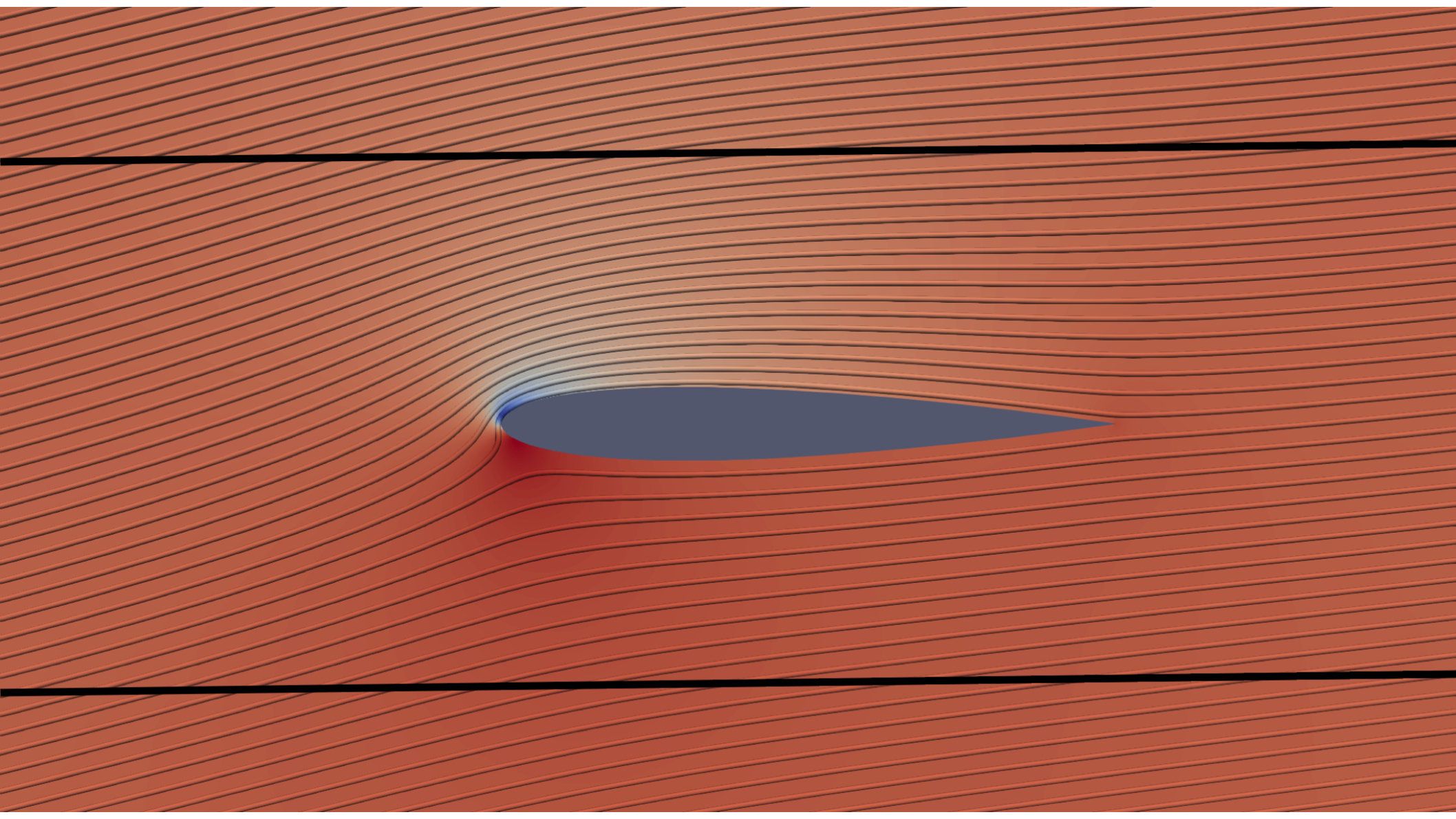
Figure 7: Pinched streamtubes at the top of the airfoil 364554 — Pressure distribution shown

The next theory on the list is the so-called **streamtube pinching. Figure 6 shows the principle of this ansatz which argues that we have constricted flow on top of the airfoil and unconstricted flow beneath the airfoil which, according to Bernoulli’s equation, again should show that higher velocity induces low pressure and vice versa again resulting in lift.

The problem with this explanation is that an airfoil in a big open environment does not really care about the pinching about streamtubes and extended flows do definitely not behave like nozzles. With that logic, a flat plate with a positive angle of attack would also experience no lift (figure 7).

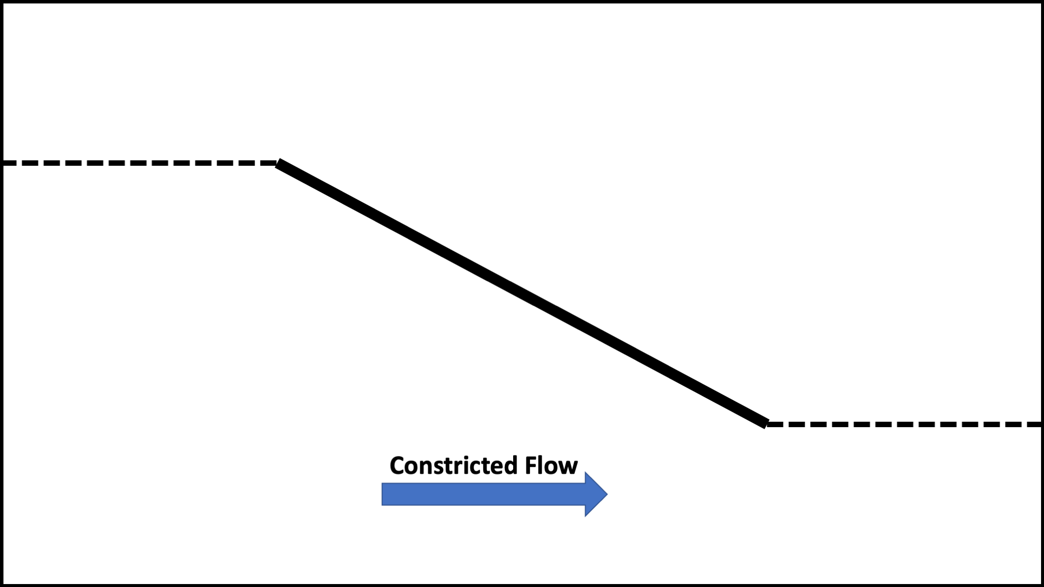
Figure 8: Pinched streamtubes for a flat plate for positive AoA

\underline{\textbf{4. Popular good explanations}}

\underline{\textbf{4.1 Flow turning}}

One of the better theories out there states that the flow passing the airfoil is deflected downwards, also affected by the shape of the airfoil and AoA. Physically explained, the downward turning of the flow requires an acceleration of the flow which induces forces:

Airfoil must push down on the air (Newton’s 2nd law)
Air must push the airfoil up (Newton’s 3rd law) which generates lift

These points take into account the behavior on the surface of the airfoil and do not answer the question of how the flow that touched the surface actually gets imparted into bigger areas of air.

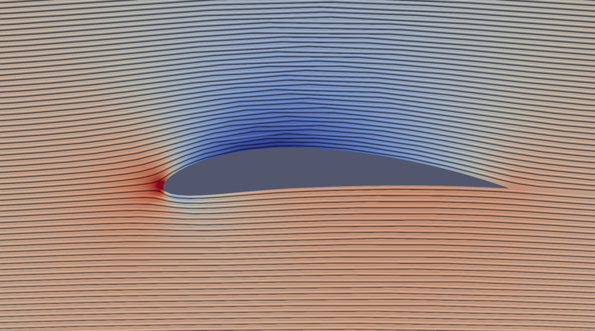
Figure 9: Downward turning flow on the upper surfaces of the airfoil — Pressure distribution

\underline{\textbf{4.1.1 Parenthesis: Newton vs. Bernoulli}}

A lot of people argue that either the theory involving Newton’s law(s) or the one with the explanation of velocity and pressure relation following from Bernoulli’s equation is right. Both explanations are satisfactory but not complete. A “complete explanation needs to look at both theories”, as Doug McLean, a retired Boeing Technical Fellow, puts it.

“Bernoulli” handles the near field of the airfoil concentrating on the surface pressure and the velocities outside the boundary layer.
“Newton” takes into account the whole swath of the flow dealing with momentum flux and flow direction

where both points are not at all contradictory but rather complementary as stated above.

\underline{\textbf{4.2 Streamline Curvature}}

We will start introducing this theory by having a look at a fluid parcel moving along a streamline with a pressure drop in the x direction, meaning that

\frac{dp}{dx}<0 \tag{4}

and if the pressure increases along the streamline, our fluid parcel will decelerate—Bernoulli’s equation describes this mathematically (derivation at the end of this paragraph). Here we can see that applying Bernoulli’s equation can only be done along a streamline and not take into consideration several streamlines and explain pressure and velocity changes.

Figure 10: Fluid parcel moving along streamline

Now let’s consider a curved streamline as depicted in figure 11.

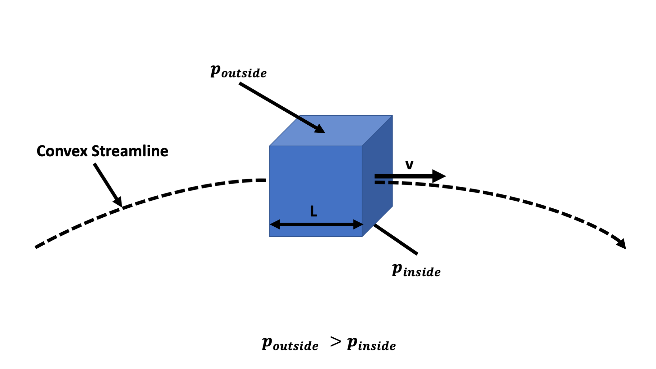
Figure 11: Fluid parcel moving along curved streamline

In order for the parcel to stay on the streamline, it is necessary that there is an external force, namely centripetal force, that is acting on the fluid volume which can only exist if there is a pressure difference.

That leads to the conclusion that if a streamline is curved, there has to be a pressure gradient across the streamline. Furthermore, the pressure is increasing the further away from the center of curvature we are!^1

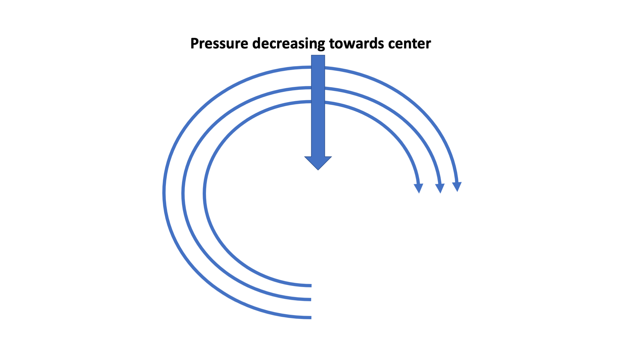
Figure 12: Streamlines and pressure gradient in a vortex

Picture 12 graphically demonstrated a vortex (or analogously a tornado) consisting of concentric circles of streamlines. As previously mentioned, there has to be a pressure gradient across the streamlines with pressure dropping as we get closer to the vortex core and the velocity increases, which explains why a tornado sucks objects towards the sky. ^1

\underline{\textbf{Mathematical Derivation}}

Consider the same fluid parcel with a pressure at the rear and front where

\frac{dp}{dx}<0 \tag{5}

meaning that the parcel is pushed from the left to the right side.

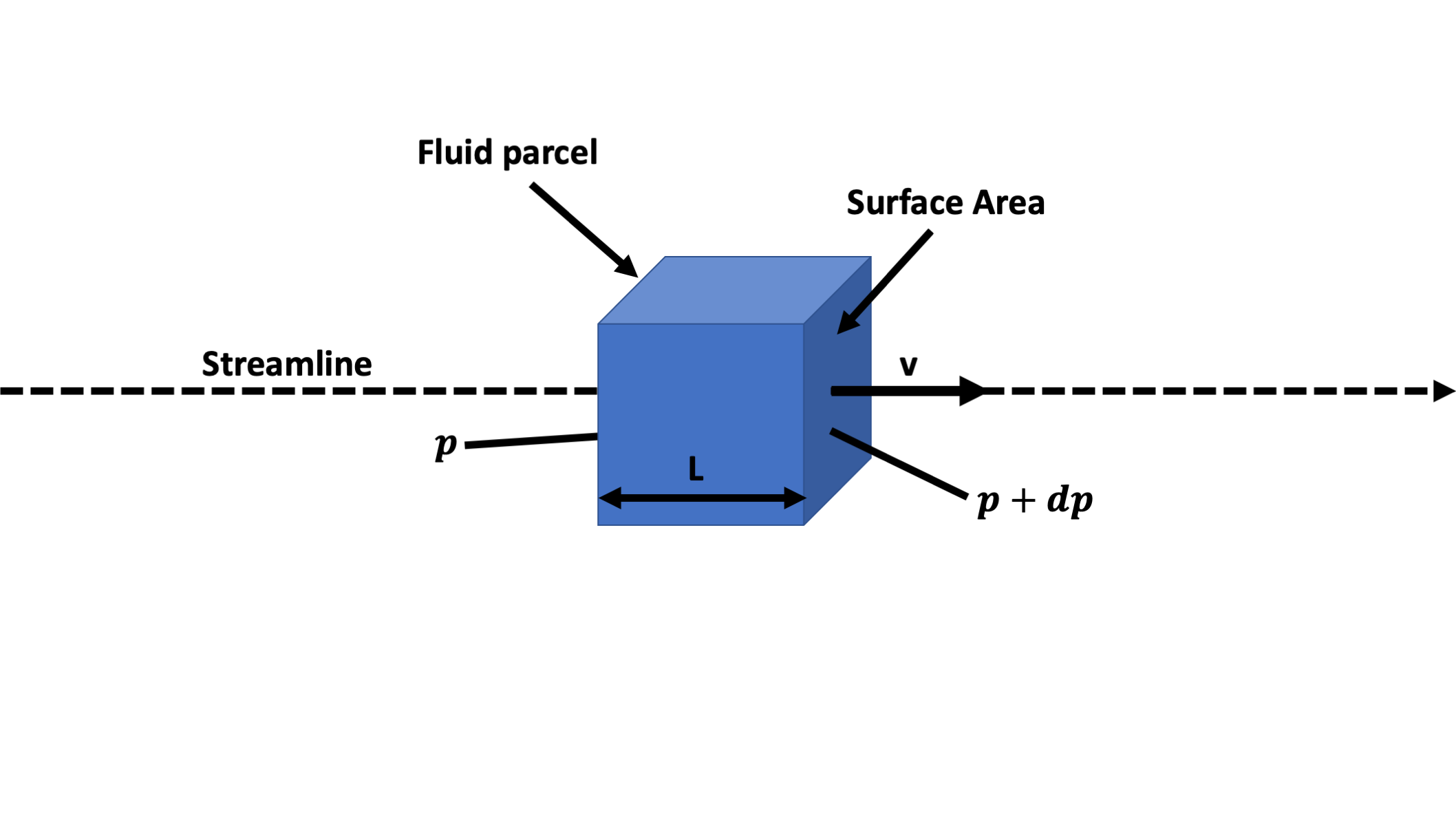
Figure 13: Fluid parcel with relevant parameters

We start with Newton’s 2nd law

F = ma = m\frac{dv}{dt} \tag{6}

and the pressure force which is defined as

F = -dp A \tag{7}

The minus in front of the differential pressure is negative as the pressure acts against the positive (from left to right) x-direction. The mass of the fluid parcel is very easy to determine

m = lA\rho \tag{8}

The magnitude of the pressure change between the front and rear can be determined from the pressure gradient in the streamwise direction \frac{dp}{dx} and the size of the parcel:

dp = l\frac{dp}{dx} \tag{9}

Combining equations 6 to 9 gives

-l\frac{dp}{dx}A = lA\rho\frac{dv}{dt} \tag{10}

which can be rewritten as

dp= -\rho\frac{dv}{dt}dx \tag{11}

Knowing that \frac{dx}{dt} is v we get

dp= -\rho \, v\,dv \tag{12}

Integrating along two points of the streamline we can determine the pressure difference

\int_1^2 dp= -\int_1^2 \rho \, v\,dv \tag{13}

p_2 - p_1 = -\left( \rho\frac{v^2_2}{2} - \frac{v^2_1}{2}\right) \tag{14}

which can again be rewritten as

p_1 + \rho\frac{v^2_1}{2} = p_2 + \rho\frac{v^2_2}{2} \tag{15}

where point 1 and 2 are arbitrarily chosen along the streamline and it is irrelevant if the streamline is curved. For the final conclusion, we have to again look at figure 11. From your physics course, you may remember that the centripetal force is defined as

F = \frac{mv^2}{R} \tag{16}

and say that the pressure on top of the fluid parcel is the pressure p plus an additional pressure that keeps the parcel on track dp thus p+dp and the inside pressure is defined as p only.

As we mentioned earlier, the mass is m = \rho \,A \,h and, additionally, we need to know that dp = h\frac{dp}{dn} where n is the direction perpendicular to the streamline (pointing away from the center of curvature). If we put all the equations together we get

F = A \, dp = Ah\frac{dp}{dn} = \rho Ah\frac{v^2}{R} \tag{17}

which yields the final equation

\frac{dp}{dn} = \rho \frac{v^2}{R} \tag{18}

which is nothing else than the pressure gradient across streamlines in terms of the flow velocity v and the radius of curvature R. For R \rightarrow \infty we have a straight streamline thus zero pressure difference—so no pressure differences across straight streamlines!

\underline{\textbf{Conclusion}}

You draw the streamlines first and then explain the pressure difference!

\underline{\textbf{5. Only Low and High-Pressure Regions}}

We now meticulously derived the mathematical expression to explain pressure differences across streamlines and know where we have high and low-pressure regions when looking at curvatures of streamlines. Another important thing to keep in mind that it is not just “low pressure on top” and “high pressure on the bottom” of the airfoil but rather separate regions (figure 14) we have to distinguish.

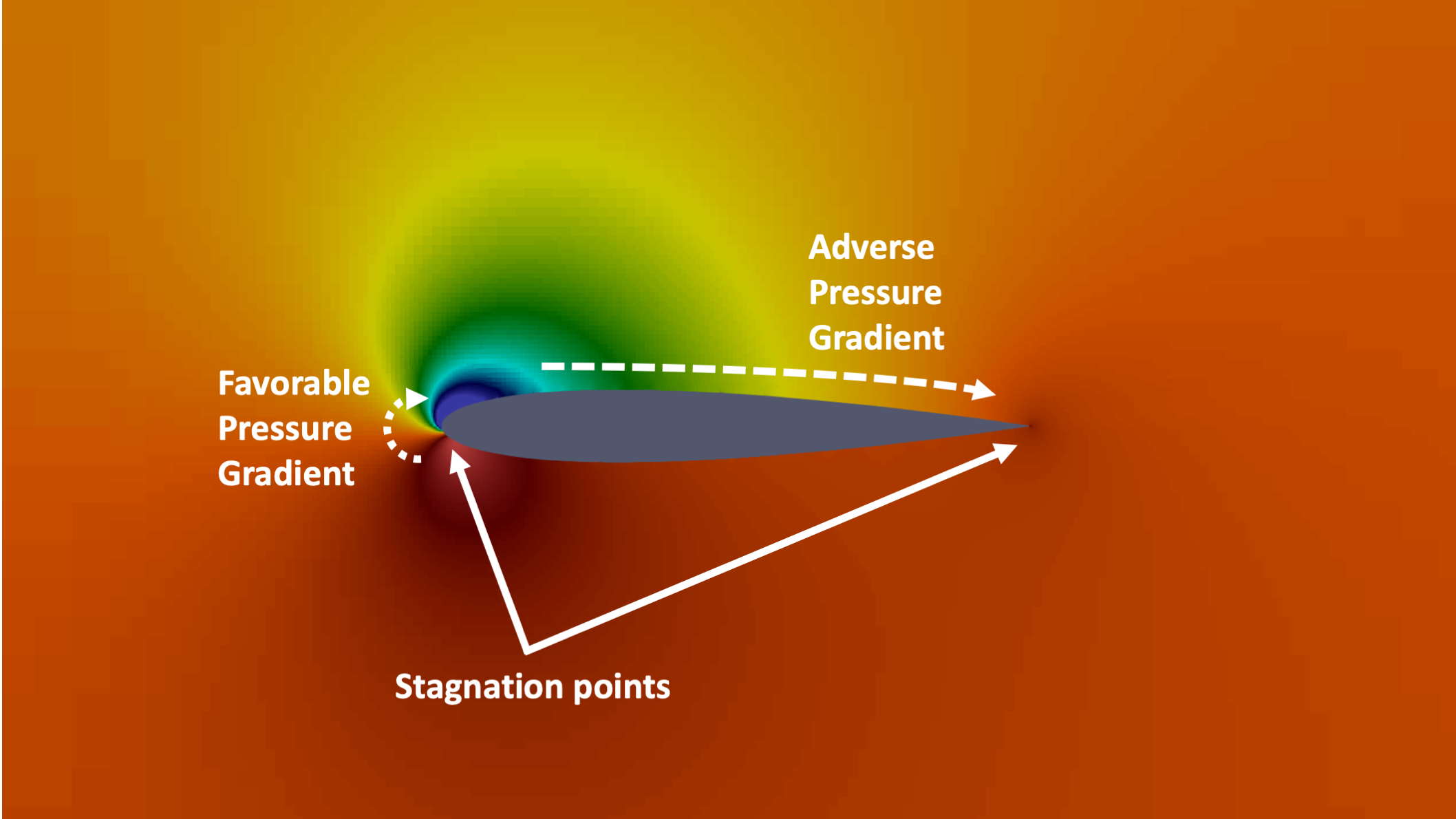
Figure 14: Cambered airfoil and regions of pressure (low pressure region in blue)

In future SimWiki articles, favorable and adverse pressure gradients will be discussed in more detail.

\underline{\textbf{Related Topics}}

Turbulence – The Gordian Knot
What is Aerodynamics?
What is Laminar Flow?
Fundamental Equations for Fluid Mechanics

\underline{\textbf{Resources}}

\underline{\textbf{Picture References}}

Figure 1: Airfoil - Wikipedia
Figure 2: File:Ray Flying Legends 2005-1.jpg - Wikipedia
Figure 4: https://www.chegg.com/homework-help/questions-and-answers/pull-blank-piece-paper-exam-book-hold-one-ends-blow-air-horizontally-top-paper-shown-figur-q17365027
Rest of the figures either done with Paraview or PowerPoint

\underline{\textbf{Literature References}}

^1 Paper from Holger Babinsky – “How do wings work?”
Krzysztof Fidkowski – How Planes Fly

\underline{\textbf{Acknowledgement}}:

I am deeply grateful to Barry Ho (@Get_Barried) for his impetus and edit of the text.