Porous Media Simulation Guide For FSAE Radiator

dschroeder · January 23, 2020, 1:41pm

I would like to start a new thread about simulations of Porous Media. I have already gone through other threads and projects, as well as other research but i feel that there is not a very clearly stated instructions on how to perform this simulation type, specifically for an FSAE car radiator.

Edit!! I was unaware of these article in Simscale that perfectly describes this process!!

Simscale documentation > Knowledge Base

Through this thread i would like to solve the following:

The correct Darcy-Forchheimer equation and how to use it.
How to calculate intrinsic and inertial permeability coefficients
Where the source of information for the above mentioned calculations comes from
Understanding the specific simulation condition to achieve correct results

My status so far:

Source of Equations from OpenFOAM: DarcyForchheimer - OpenFOAMWiki

The Darcy-Forchheimer Law states the following:

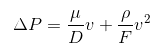
Where:

D is the Darcy coefficient - Also known as Intrinsic permeability

F the Forchheimer coefficient - Also known as Inertial permeability

Simplifying this equation we get:

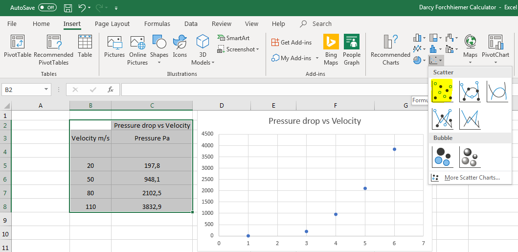
From here we need to input our values from the pressure drop VS Velocity curve.This can be made in Excel from the raw pressure drop VS velocity data.This data should be given to you (or asked for) from the radiator manufacturer.

Ric has recently sent me an amazing video on this topic Fluid Mechanics 101: Porous Media

In our case, the manufacturer AKG did a workshop with our FSAE team and also provided simulation software for the radiator. This provided the following data.

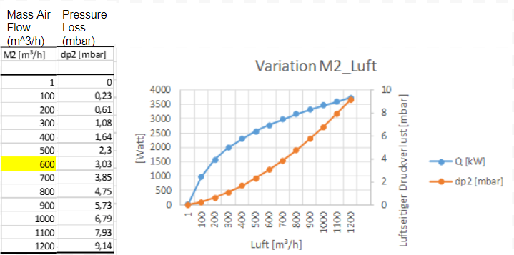
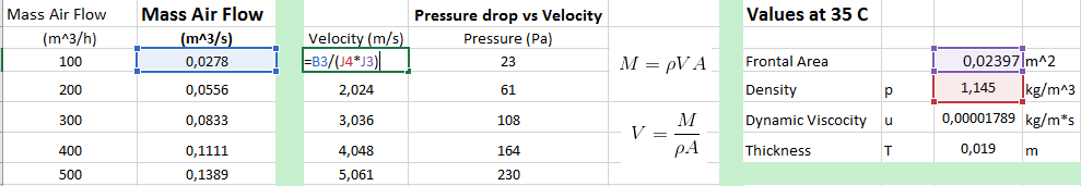
In my situation, the Mass air flow is in meters cubed per HOUR. This means it is important to check your units so that the results make sense. Since we need our Mass air flow in M^3/S we must divide the data by 60 to get minutes then 60 again to get seconds. Using Excel makes short work of these calculations by using an equation to relate the MAF data input. Then dragging this equation down, calculates each result using each new input.

Now using Mass Air Flow in m^3/s we need to convert the mass airflow into velocity using the following equation.

ρ: Density of the gas, in kg/m^3

V: Flow speed, in m/s

A: Flow area, in m^2

M: Mass flow rate, in m^3/s

Using excel, we can equate this conversion to get our final Velocity in (m/s) Vs Pressure Drop in ¶. Pressure data was recorded in mbar so we must just multiply these values by 100 to achieve Pa.

For simplicity i have used an example graph and curve equation output from hypothetical data.

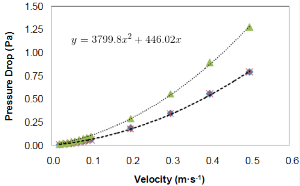
The graph then outputs the velocity dependent pressure values in the example equation shown:

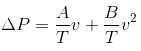
Switching the x and x^2 components of the equation gives us the comparison to the simplified Darcy-Forchheimer equation and lets us calculate the coefficients.

The inputs for A and B come from the curve fit equation produced from the graph

Simplified Darcy-Forchheimer Equation

Where

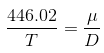
A = 446.02

B = 3799.8

Resulting in
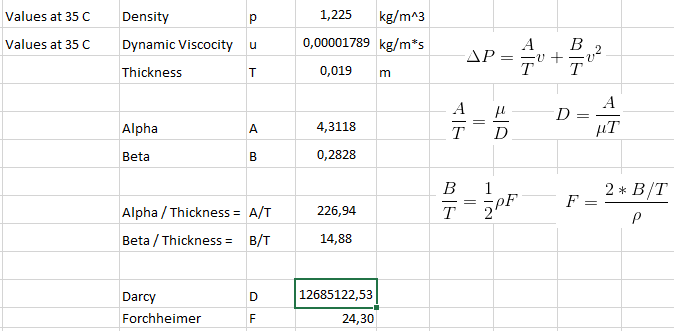
In the case of applying this equation to porous media, the simplified variables A and B must both be devided by the thickness of the media in that specific direction. This produces the following equation:

Where

T = Thickness of Porous Media (direction dependent)

Knowing the velocity dependent pressure values, we can calculate A and B and thus, the coefficients and can be recalculated. It should be clear, that the vectors and can be direction dependent.

Solving for the needed coefficient D results in the following:

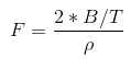
Following this procedure will give you the Darcy and Forchheimer coefficients for the porous media input parameters.

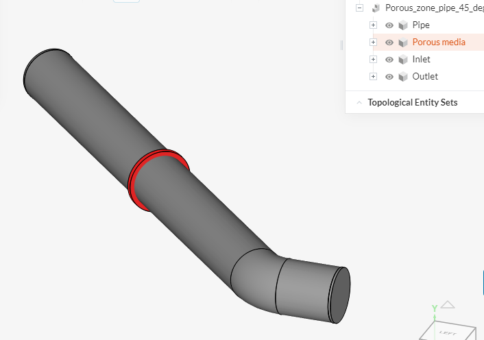
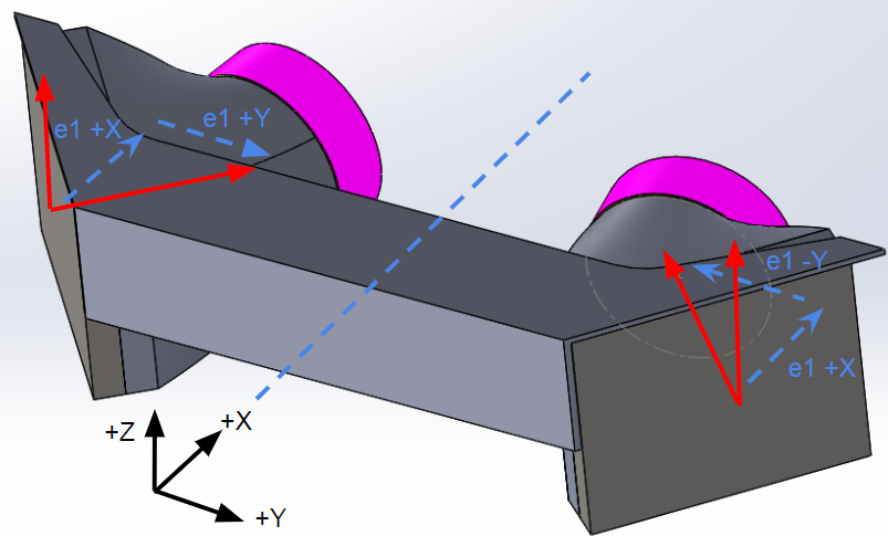
Now that we have the coefficients we have to input their direction through the vectors e1 and e3. With the flow U moving along the positive X axis, The first vector to find is e1. In the example provided by the Simscale FSAE tutorial, the radiator is tilted by a certain angle, but the front face is parallel to the Y axis, meaning there is no Y component to the e1x, e1y and e1z coordinate system. So e1y = 0.

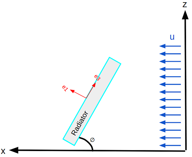
In my situation, the radiator face is parallel to the Z axis, so my e1z component will equal 0. e3, as explained in the tutorail is perpendicular to e1, so in my case e3z will equal positive 1 giving the direction in the z axis.

The e1 vector is calculated by creating a coordinate system around the point. As said above, e1z =0 because the radiator face is parallel to the z axis. To calculate the angle and direction, measurements were taken from the 3D model. The values are not important, as long as the X and Y components equal the 50 deg angle of the radiator as shown below.

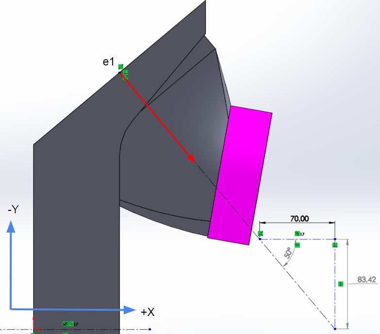
Here we have a value of 70 in the positive X direction, therefore e1x = 70. With an angle of 50 deg, this creates a Y component value of 83.42. By leaving this value positive, it determines that the radiator face is pointing towards the centerline in the +Y direction. For the other side of the car, in a full car simulation, this value must be negative to show the radiator face is pointing in the opposite direction.

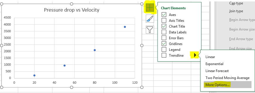
How to create a Curve fit graph for Darcy-Forchheimer calculations in excel

In order to calculate the coefficients, we must relate our pressure drop VS velocity data to a second order polynomial. This can be done easily through excel.

Input the data as shown below in two columns with a title. Then select the whole data set and input a scatter plot graph.As you can see our pressure data is represented on the vertical axis but velocity isn’t,

Simply select the data set on the graph and drag the purple and blue boxes to represent only the numerical data. We now have our data plot.

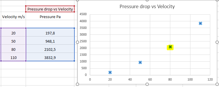
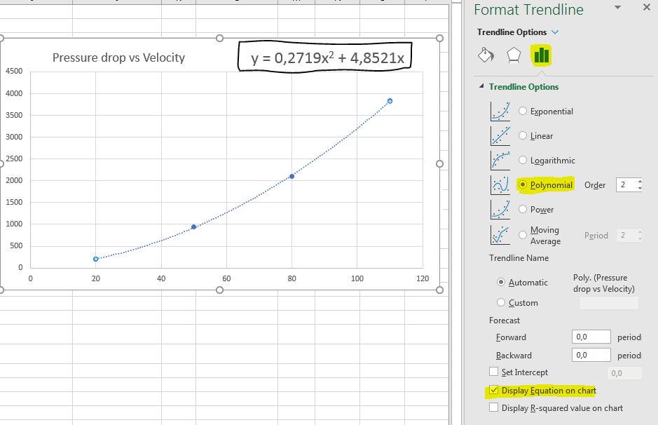
Then under the + tab selection next to the graph, select the arrow under trendline then more options.

Navigate to the three bars under trendline options. Select Polynomial for line type. Then select Display Equation on chart. You will now see the function that is used to relate the Pressure drop VS Velocity data to the Darcy-Forcheimer equations. In this case Alpha (A) is 4.851 and Beta (B) is 0.2719.

Adding the equations and relations between them into excel helps to further automate this process.

Good Luck!

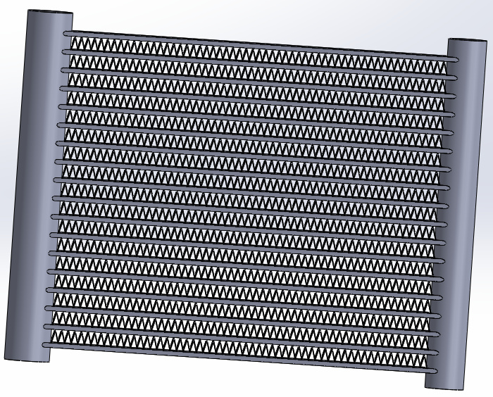
Obtaining pressure and velocity data from self-made Radiator Simulation

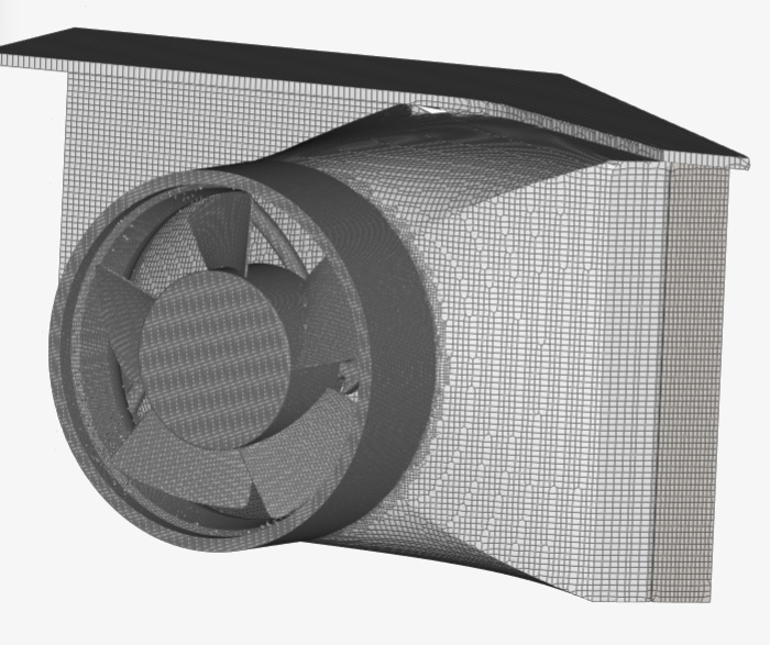
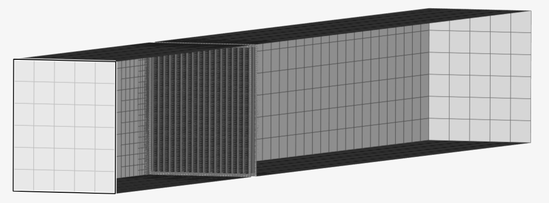
It is also possible to simulate the pressure drop using the real radiator model and achieve the Pressure Vs Velocity data. To set up a simulation. First create a wind tunnel that completely encloses the radiator porous zone.

Simplified radiator Geometry with border

Bounding Box Encloses radiator porous face

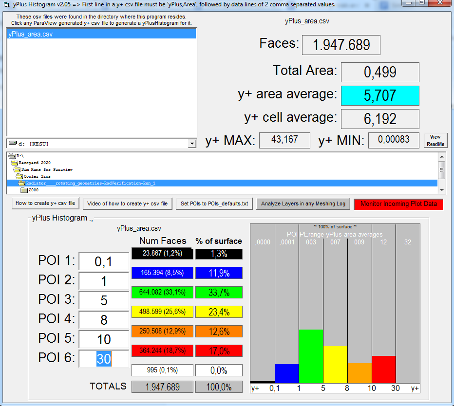
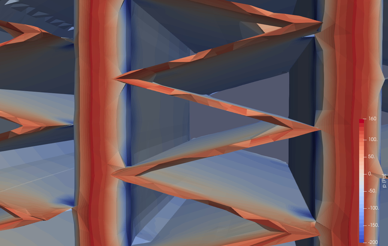
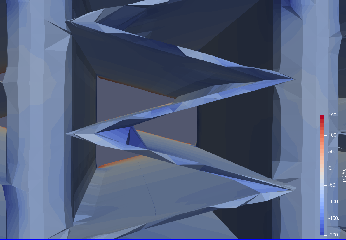
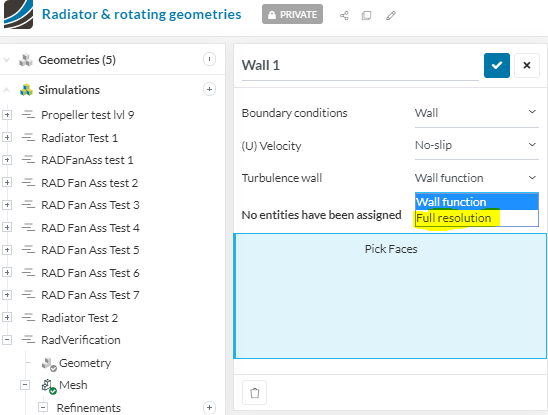
The best method to measure pressure drop across the radiator fins is with the viscous sublayer (Y+< 8). Due to the small size of the fins and the space between them, the shear forces are the greatest factor for this pressure drop. There is undoubtedly inertial forces at play, but any boundary layer formed in these tight areas, and over such a small distance (20mm thick) will be mostly laminar and not turbulent flow. My simulations are run using the K-Omega SST model but using full resolution (for laminar flow Y+=< 8) and not wall functions (for laminar approximation and turbulent flow - Log-Law region 30 <Y+< 300).

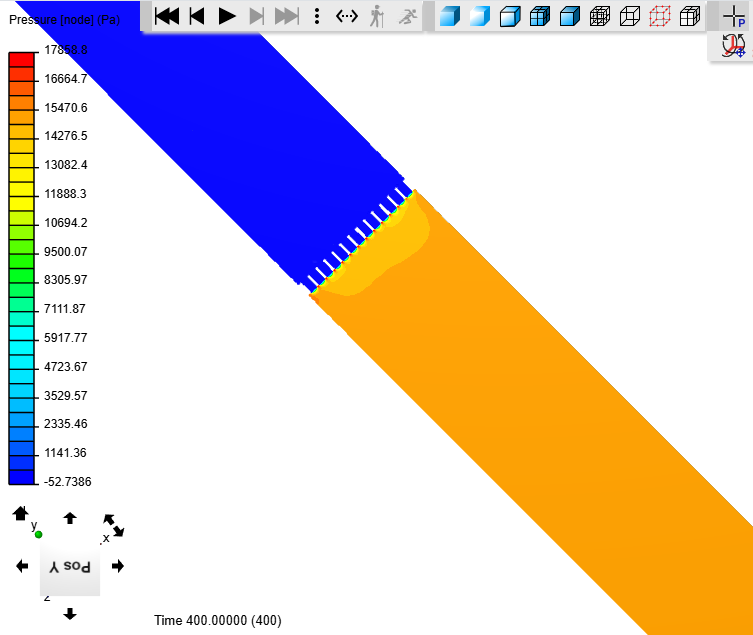
Pressure Drop Data selection

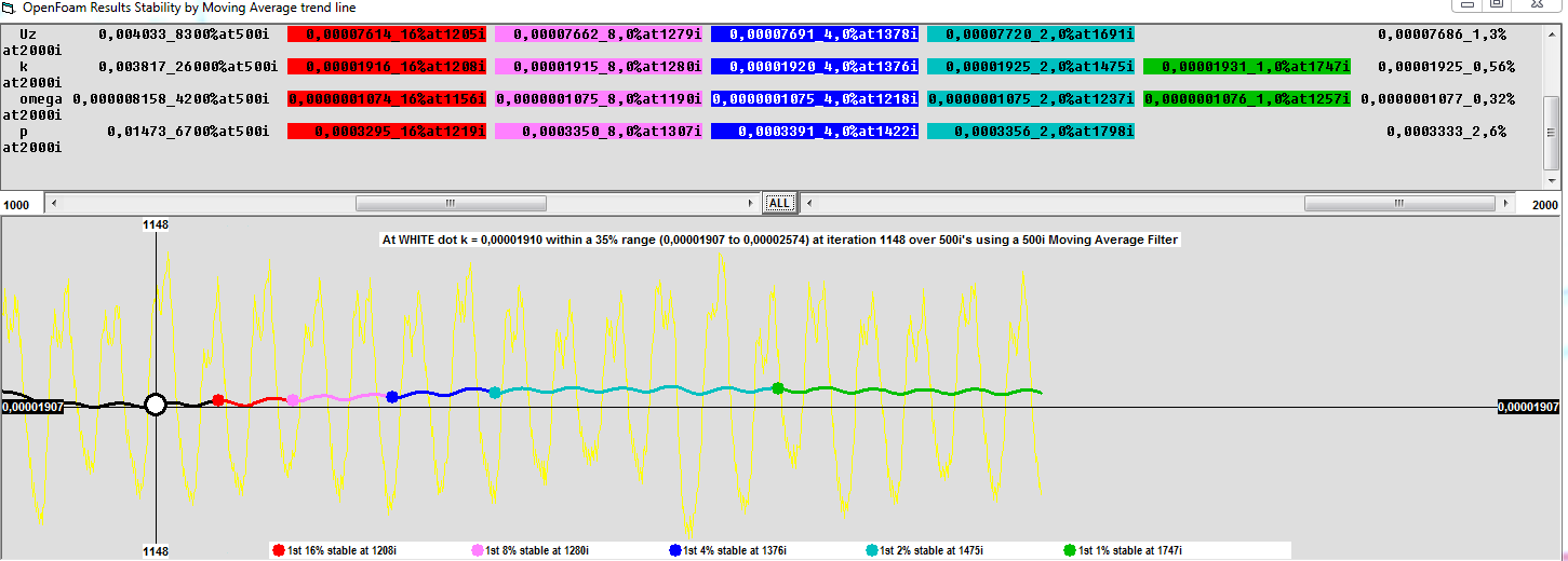
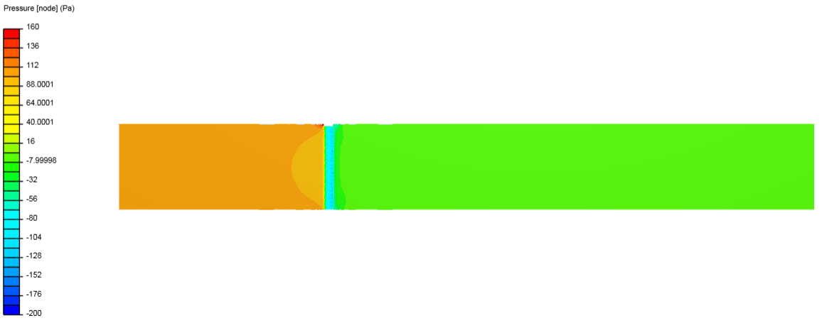
After the simulation is complete and Y+=< 8 values are verified, the resultant should look something like this.

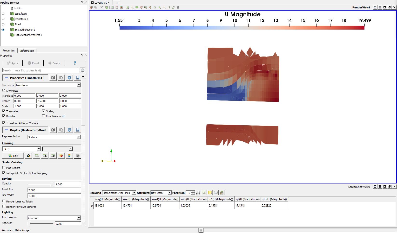
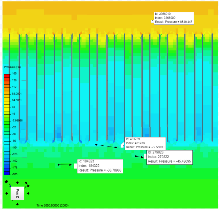
Upon closer inspection the pressure zones can be identified.When a slice is made through the middle of the radiator, you can use the “Select Element” tool from the top toolbar in Simscale. This allows you to click on every HEX prism and find the node data from that point.

My overview slice of the radiator shows

Dark Orange ~ 100Pa - inlet starting pressure at 10m/s velocity setting

Light Orange ~ 96Pa - pressure starts to drop as the air speeds up to pass through the restrictive fins (Bernoulli effect)

Dark Green~ -10Pa - pressure drop after passing through the radiator - pressure recovery zone

Light Green ~ -3Pa - Final pressure difference

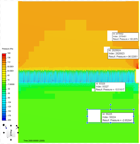
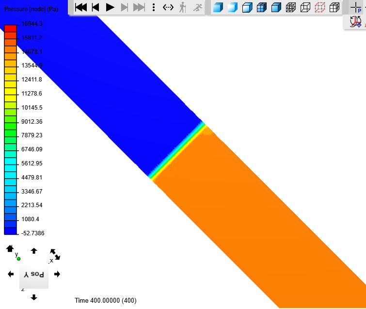
The data to be collected is going to be the pressure values that are present upstream and downstream of the radiator. This will give us the total pressure difference of the system. Data taken too close to the radiator will give an incorrect representation of the results. This is best said by Ricardopg later in the thread.

“If you make a slice immediately downstream of the porous zone, this area is most likely going to have the lowest pressure fields. As you go a little bit further downstream, flow recovers some pressure as it readjusts (Bernoulli).For the porous zone formulation, pressure drops are permanent - there’s no recovery. So if you don’t take the aforementioned recovery into account, you will most likely end up with a pressure drop that is bigger than the one you would expect.”

So our pressure drop data to be used in this case, would be:

Starting Pressure 100Pa - Ending Puressure -3Pa for a total difference of 103Pa

Velocity Data selection

Now for the velocity data, based on the video earlier in the post, the data should come from the air speed directly in front of the radiator face. This is shown below. Again the “select element” tool is used to collect the node data. We see here that our starting inlet velocity is 10m/s and continues to increase before the radiator face as the air speeds up. We will be taking the data from the dark orange area, which has increased to about 11m/s.

Velocity profile

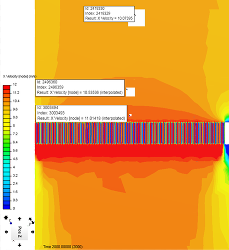
We now have our first input for our Pressure drop vs velocity data set. By simulating at multiple speeds we can get a range of values to be used in the Excel program to calculate the Darcy-Forchheimer coefficients.

Pressure drop Pa	Velocity m/s
103	11

Please comment on the equations and methods i have listed above. I want to know if what i am doing is accurate or even correct.

I will upload results once i get the velocity VS pressure drop data from the manufacturer.

Thanks, Dan

jousefm · January 23, 2020, 3:02pm

That’s awesome Dan!

Funny because I found the same video few days ago and planned to do a video on how to implement this in Matlab or Python Thanks a ton for your efforts

Jousef

dschroeder · January 23, 2020, 3:42pm

A excel program with inputs would be awesome to have. Once i get the data from either a teammate or the manufacturer i will be working on that.

Otherwise does my method look good? Its always nice to have conformation on these things

Ricardopg · January 23, 2020, 3:51pm

Hey Dan,

For porous media, I believe the best way to answer these questions is by validating a case, e.g. comparing a perforated plate (the real geometry) to the porous medium simplification.

The formulas you posted are almost correct. You need to divide the right hand side of both D and F formulas by the thickness of the porous medium in that specific direction (do an unit check). Later, d and f calculated will be the input. There’s no need to use the inverse.

OpenFOAM accepts negative values for d and f, but it will basically use this number as a multiplication factor for the biggest positive d or f factors that you used (in the case of an anisotropic medium).

/Ric

dschroeder · January 23, 2020, 4:06pm

Thanks Richard!

I assume you mean thickness as in the width of the medium and not the cross sectional area. So my radiator is 34mm thick. This is the value correct? I just want to be sure as i have seen some equations say thickness, then the description they give is actually for area.

Ok so i dont have to worry about negative numbers in Simscale? Ill just leave it as is then.

Also thanks for uploading pictures of your validation case. I assume based on the pictures that the bounding box perfectly seals around the medium you are testing correct? Here is the simplified radiator part

Any recommendations on simulation setup?

Ricardopg · January 23, 2020, 4:34pm

I assume you mean thickness as in the width of the medium and not the cross sectional area. So my radiator is 34mm thick. This is the value correct? I just want to be sure as i have seen some equations say thickness, then the description they give is actually for area.

It’s thickness (or width, length, as you prefer) in units of meters. When you define your porous medium, you will set a local coordinate system. This thickness would be the thickness of the porous medium in each one of the local directions.

Yes, the porous medium covers the pipe entirely. The geometry looks like this:

Any recommendations on simulation setup?

Well, the best option would be to work with data directly from the radiator supplier. Maybe you can find an empirical approximation formula for the forchheimer coefficient… it would be an approximation, of course.
For instance, there’s an approximation for the forchheimer coefficient for perforated plates called Van Winkle equation, where you estimate f based on the total area of the plate and total area of the holes.

And you can also use the d and f coefficients provided in one of the fsae tutorials as an approximation.

dschroeder · January 23, 2020, 4:49pm

Ok thanks for the info. I will update my equations.

For my bounding box sizing, i can just make something that will fit exactly around the Lamelle and cross tube area

I agree with this, as simulating the actual radiator would give me the velocity vs pressure drop data, but i would have to do multiple simulations. The real world data is better to measure the coefficients with.

I would prefer to either get the manufacturers data or simulate myself. I wouldnt want to pull data from the tutorial, which most likley has a medium of another thickness. this would make the results not that accurate.

What I may try is to run the mesh i already have done with the tutorial D and F values as i have a MRF zone fan to test as well. the results wont be correct but i can see if the simulation is working as intended.

dschroeder · January 27, 2020, 6:08pm

So an update on this project and a few questions.

I am not sure if I am simulating this correctly or not. My initial assumption is that the best method to measure pressure drop across the radiator fins is with the viscous sub-layer. Due to the small size of the fins and the space between them, I am guessing that the shear forces are the greatest factor for this pressure drop. There is undoubtedly inertial forces at play, but any boundary layer formed in these tight areas, and over such a small distance (20mm thick) will be mostly laminar and not turbulent flow.

Now, In my full car simulations I am using the K.Omega SST Turbulence model. This radiator test is only meant to give me the pressure drop vs velocity data to be used in the Darcy-Forchheimer equations. In the end, any results measured from the porous media radiator on the full car will use the K-Omega SST model. Onto my questions:

If my above assumption is correct about measuring the laminar flow, Should I still be using the K-Omega SST Model?
If so, can I simply choose full resolution when assigning the no-slip wall condition to the radiator model as shown below?

In order to collect a data range, i will be simulating at different speeds. However there are many other variables to consider. Comparing my results with the manufacturer’s data is important to validate the tests. If I am somehow unable to get the manufacturers data, I do have some data, such as water and air inlet and outlet temps. My questions about this are as follows:

To get accurate Darcy-Forcheimer coefficients, Should the air temperature value within the bounding box, and therefore density and dynamic viscosity values, be equal to the radiator air inlet temperature provided by the manufacturer (35 C) or ambient temperature values (20 C)?
Is there any way to pre-set the temperature of the geometry itself? The Water temperature through the radiator is naturally different at the inlet and outlet but this would be too complicated and i would be satisfied with an average over the whole surface.
In addition to #2, is it possible to preset a temperature within the porous media?

If I am able to get the Velocity VS Pressure Drop Data from the manufacturer, the data will come from a controlled environment, with the radiator perfectly sealed, no turbulence, aligned with the incoming air, etc… this is scenario is shown in my current wind tunnel setup shown below.

Would It be better to collect the velocity Vs pressure drop data in a scenario more similar to how it is built on the car? (50 deg angle off the centerline of the car) I am not sure how much this will affect the results.
Would it be better to use velocity seen at the radiator face when simulated on the full car vs preset speed values? This would give actual radiator face air speeds due to affected wing geometry and car turbulence.

I apologize for so many questions. I am trying to obtain accuracy in my results without too much overkill. If there is anything mentioned above that is totally unnecessary to worry about just say so. Also such questions, and hopefully answers, might help others trying to decide/understand what is important in such a simulation.

Ricardopg · January 28, 2020, 2:40pm

Hummm… for the first set of questions, I guess you can try to run using k-w sst and laminar to see how different they are. And yes, you can of course use full resolution, just keep in mind y+ requirements.

For the second set: temperature is not taken into account in incompressible simulations, so I’d just stick to ambient temperature for the sake of simplicity (but you can always run sensitivity tests!).

For the third set: you will set a local system of coordinates when you set up your porous media. This video shows the velocity of interest at around the 7-8 minutes mark.

dschroeder · January 28, 2020, 9:30pm

Ok If i have time, I will try both models. Maybe the full resolution within the k-Omega SST will be accurate enough though. My Y+ = 1 with an attempt to use only 1 layer as Dale and I have done on previous simulations. I’m not sure if a 1 layer BL applies to laminar flows but i will give it a try. I have also used the Y+ Histogram program from Dale to see if the Y+ values are where they should be.

This shows an OK Y+ area average of 5.7 but I would like to reduce this more. What is not ok, is that there are cells above Y+ of 8. I will be running another simulation to see if i can get all cells under this value.

Inflate boundary layer settings - layer calculation		Y+ Value
Layers	1
1st	0.00001512	Y+ = 1
Overall thickness	0.00001512
Expansion ratio	1
Min thickness	0.000001m
Reference Length	0.02m

The results from the ORSI calculator provided evidence of stability in the simulation. I will run further simulations until about 1800 iterations.

Ok, so there is no possibility of adding a temperature preset to the radiator. However, the air density and viscosity values are changing depending on the temperature. I think it is best to use the manufacturer data for air inlet temperature. If the simulation cannot estimate the increase in air temperature over the radiator, and therefore density and viscosity changes, then the ambient temperature will account for this.

The video you sent me was extremely useful, especially when it stated that the velocity data should be taken from the radiator face and not the user defined velocity when compared to pressure drop data.

Is there a way to get graphical data of the face velocity? In one of your posts i saw something on the Average Area or Average Integral result control. How would I apply this to my radiator face? Would i have to select every single front fin face to insert into the assignments box?

Ricardopg · January 29, 2020, 2:26pm

For this test that you are making, wouldn’t it be equal to the inlet velocity? There’s no way for the flow to go around the radiator, it has to go through the fins

dschroeder · January 29, 2020, 4:53pm

For the test yes, it would be equal. This is the question,

Do i make the inlet velocity of the test the same speed as the cars velocity, as in 10, 20, 30 m/s

or

Do i make the inlet velocity close to the “Local” velocity at the radiator face. This would mean if the cars velocity is 10 m/s for example, that after the air passes through the wings, gets all mixed up in turbulent flow, the velocity at the face might be 8 m/s, or could be higher, like 11 m/s based on its location on the car.

Based on the video you sent me, i think the Local velocity is better to use, however i am not sure of how to get this exact result. I can always use post processing to estimate the face velocity based on the color variations on the radiators surface, but i was hoping for a better method.

DaleKramer · January 29, 2020, 6:51pm

If I understand what you want, this might get you there…

You can do this in ParaView to get the average of a selected set of cells…

Transform Filter to rotate internal mesh to angle of interest (50 degree in your case)
Slice that rotated mesh to a distance in front of radiator where average U magnitude is to be determined.
Use a selection tool to select the cells of interest on that slice…
Extract the selection.
Plotselectionover time
In spreadsheet view on the filter of #5 (RowData), select only the max, min, avg etc of the parameter of interest…

.
.

dschroeder · January 29, 2020, 7:39pm

Yes that method seems like it would work well. Thanks! I wish i knew Paraview that well , seems like it can do anything!

DaleKramer · January 29, 2020, 7:44pm

Yep, and the more you use it, the easier it is to do something, that you could only dream of before

For instance, I had never done the above before, but with a small bit of Googling, combined with my existing ParaView knowledge, I had that procedure in about 10-15 minutes…

dschroeder · January 29, 2020, 7:59pm

Yea what you did seems not possible. The incoming data is from a straight on simulation, so velocity and pressure drop should be measured in that direction. You can rotate the internal mesh so that its as if I had simulated the radiator at 50 deg? I would think that it wouldnt work unless the simulation itself was of a radiator at 50 deg

Im going to try this now with the first simulation that worked. As shown in the previous posts the Y+ values werent that good. I have two more meshes running with the 1 layer BL at 1.0e^-5^m and 7.5e^-6m. Lets see if those will work. Ill upload the pictures of your method if i can get it to work

DaleKramer · January 29, 2020, 8:06pm

Yes, one big trick there is to do that rotation for ease of selection. The rotation should not affect the U magnitude as that is not a vector and has no direction associated with it… Maybe there is a way to select the cells of interest without the mesh rotation but I do not visualize any method yet. Think about that problem and you can maybe come up with a way to select the cells without rotation… If you want to look at any vector field in the rotated and selected cells, you could always rotate the selection back to 0 deg I suppose…

dschroeder · January 30, 2020, 12:29pm

Here is the Pressure across the front face followed by the rear face. From the visual data, I would say that the front fins are at about 110-120 Pa and the rear about -60 Pa.

Pressure Front

Pressure Rear

Based on this data could I assume that the difference of Pressure is 120 - (-60) = 180 Pa? So my pressure drop across the radiator is 180Pa.

I found out that you can select a specific point in simscale an it gives node data. This shows a frontal face velocity of 8.8m/s and rear velocity at 13.5m/s. This makes sense because the increased frontal pressure should produce slower velocity air and the rear faster velocity then the input.

Therefore, for this example, would i be correct in assuming the data for the Velocity Vs Pressure drop should be:

Velocity 8.8
Pressure 180

Inlet Velocity	Velocity at Rad Face	Pressure Drop
10m/s	8.8m/s	180Pa

Front Velocity

Velocity Rear

Ricardopg · January 30, 2020, 2:01pm

I’ll point out one thing that I eventually encountered while doing my own validation. When you simulate the complete geometry, you will get much more local detail regarding pressure and velocity (obviously).
If you make a slice immediately downstream of the porous zone, this area is most likely going to have the lowest pressure fields. As you go a little bit further downstream, flow recovers some pressure as it readjusts (Bernoulli).
For the porous zone formulation, pressure drops are permanent - there’s no recovery. So if you don’t take the forementioned recovery into account, you will most likely end up with a pressure drop that is bigger than the one you would expect.

dschroeder · January 30, 2020, 4:11pm

Ah ha, thanks for the tip! I wasnt sure exactly what to look at due to not knowing exactly how the simulation handles these situations. Your suggestion of cutting the surface worked really well. Combined with the “Select Element” tool in Simscale, I can click on every HEX prism and find the node data from that point.

My overview slice of the radiator shows

Dark Orange ~ 100Pa

Light Orange ~ 96Pa

Dark Green~ -10Pa

Light Green ~ -3Pa

Looking at the important areas the slice shows

Very Light Orange ~ 86Pa - This is the average value I think I should use for the inlet pressure value

Light Blue (least see through) ~ -72Pa

Light Blue (medium see through) ~ -45Pa

Light Blue (highest see through) ~ -33Pa

Now the question is which Low pressure Light blue region to use. The pressure increases quite quickly in this area. Would it be better to take the average value of pressure just before it leaves the fins? This is a fairly stable region and doesnt have such drastic pressure changes. So in the next picture I would say the pressure outlet would be around 100Pa

Also the mesh quality wasnt that great on this run. I will be re-doing this and extending the “wake” region refinement for after the radiator