Recording
Homework Submission
For your homework, your task is to investigate the behavior of drag and lift and determine the stall zone for two different front wing flap angles: 6 degrees (standard) and 18 degrees (high downforce) considering a constant inlet velocity of 20 m/s.
The step-by-step tutorial below contains all of the steps for setting up the simulation in SimScale and visualizing the results.
To submit your homework assignment, please generate a public link of your project (Sharing a Project)
Homework Deadline: The homework deadline has been extended until September, 26th 11:59 pm CEST
Click Here to Submit your Homework
Outline
PART 1:
-
Introduction
-
Project Import
-
Mesh Generation
a. Geometry Primitives
b. Mesh Refinements
c. Start Operation
d. Additional Meshes
e. Mesh Quality -
Simulation Setup
a. Analysis Type
b. Domain
c. Initial Conditions
d. Boundary Conditions
e. Numerics
f. Simulation Control
g. Result Control
h. Simulation Runs
i. Additional Runs -
Recommendations About Comments
PART 2:
-
Post Processing
a. Filters/Visualization
b. Additional Features -
Homework Link
-
Result Comparison
a. Standard vs High Downforce
Introduction
This is part one of the step-by-step tutorial. In this part you will be guided through the meshing setup and simulation setup. In the second part you will be guided through the post-processing of the results and we will visualize and analyze some results.
Lets dive in!
In this tutorial, you will be doing a full fledged flow simulation of the aerodynamics of a front wing. The focus of this simulation is to investigate the drag and lift forces on the wing and identify flow separations.
For your homework, your task is to investigate the behavior of drag and lift and determine the stall zone for two different front wing flap angles: 6 degrees (standard) and 18 degrees (high downforce) considering a constant inlet velocity of 20 m/s.
Let’s take a look at the physics of the front wing before we start to set up our simulations:
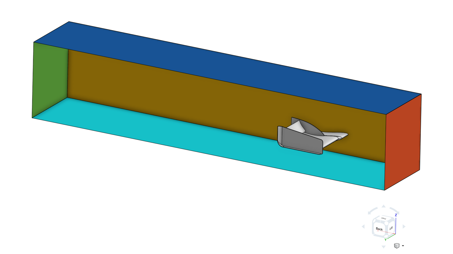
As a first simplification we can exploit the symmetry of the front wing. Simulating only half of the wing reduces the computational effort by defining the inner surrounding wall (brown) as a symmetry plane.
The body of the wing is a physical wall (grey), which means that it involves friction and should be defined as so-called “no-slip walls”.
The outer (not visible here) and upper surrounding walls (dark blue) are necessary to limit the size of the domain we want to simulate since we are not able to simulate an infinitely large domain. In reality, these walls do not exist and should not interact with the flow. A good approximation here is to assume this wall as frictionless or so-called “slip walls”.
The bounding face on the right-hand side (red) will be defined as an inlet with a constant flow velocity profile.
The bounding face on the left-hand side (green) will be defined as an outlet with a constant pressure.
These four bounding walls define the size of the fluid domain, and in general you have to reach a compromise: you want these walls as far as possible so that you can observe all the fluid behavior (also, if they are too close to your geometry you might get strange results), but you also want to limit your fluid domain to save computational power.
In reality the car is in motion, so there is no relative motion between the air and the floor. Because here the car will be standing still and the air will move around the car, to maintain the condition that there is no relative motion between the air and the floor we will apply a wall velocity on the lower bounding wall (cyan).
You will simulate two different wing set-ups for which the geometry is provided.
First we will start with the Standard Configuration and follow all the steps in detail. The other configuration(s) will follow the same procedure and therefore will not be documented in detail.
General notes:
- Most of the descriptions will be below the images.
- For many attributes, SimScale sets some default values that don’t need to be changed unless specified. Please double check your procedure with the screenshots
Project Import
To start this exercise, please import the project into your workspace by clicking on the link below:
If the project appears to be private, please make a copy of it to work on it.
Mesh Generation
For this tutorial we will work with the Standard model for which the flap has an angle of attack of 6 degrees.
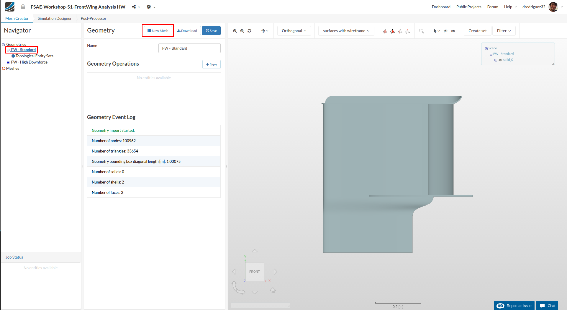
Start by clicking on the FW - Standard model under Geometries in the navigator. Then click on New Mesh to start creating a new mesh on this geometry (this doesn’t start the mesh operation, you still have to go through all the settings).
The new mesh operation will be generated automatically. Next change:
-
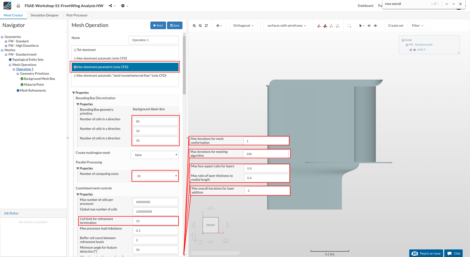
Set the Type to Hex-dominant parametric (only CFD).
-
Configure the Bounding Box geometry primitive to the following:
Number of cells in x direction to 60
Number of cells in y direction to 16
Number of cells in z direction to 16Here you are refining what is known as the level 0 refinement, or the coarsest mesh that will exist in your model. The bounding box refers to a setting you will modify in a few steps and something we already talked about in the introduction: the fluid domain. So with this you are specifying into how many control volumes you would like to split your model. SimScale generally generates a good number by default, but you are free to change it (like we do here). You have to be careful because you don’t want a mesh that’s too coarse to be solved properly but you also don’t want a mesh that’s too fine for areas where the flow is very simple.
-
Set the Number of parallel computing cores to 16
-
Scroll down to change other values to optimize the meshing parameters
-
Cell limit for refinement termination to 15
-
Max iterations for meshing algorithm to 100
-
Max iterations for mesh conformation to 1
-
Max face aspect ratio for layers and Max ratio of layer thickness to medial length to 0.6 and 0.4 respectively.
-
Max overall iterations for layer addition to 3
-
Click Save to register changes.
Geometry Primitives
Background Mesh Box
Next, under Geometry Primitives select Background Mesh Box.
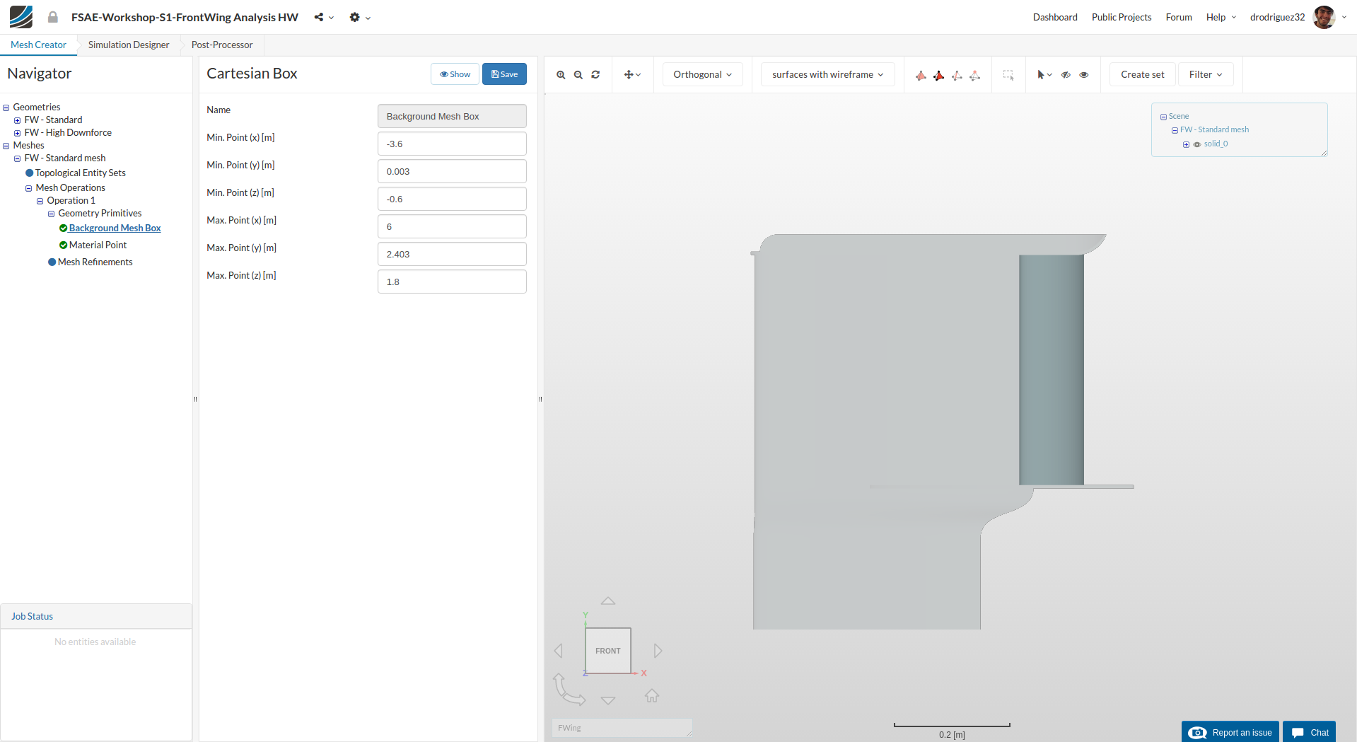
Change the setting accordingly:
- Min. Point (x) = - 3.6
- Min. Point (y) = .003
- Min. Point (z) = - 0.6
- Max. Point (x) = 6
- Max. Point (y) = 2.403
- Max. Point (z) = 1.8
Here you are defining the size of the fluid domain.
Click Save. If you don’t see the entire box click on the reset icon over the viewer to see the created mesh box.
Material Point
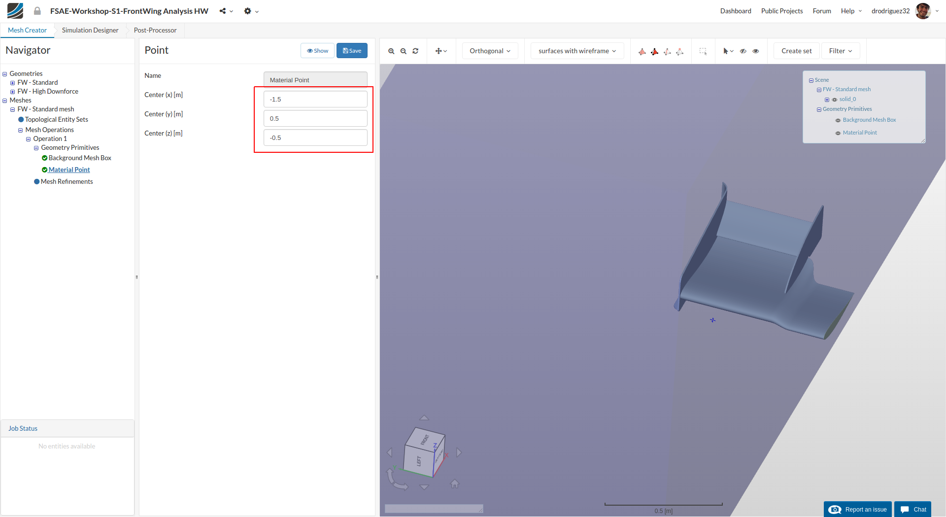
Next you will specify the material point. This will tell the platform where the mesh will be created, so make sure it is inside the Background Mesh Box but outside of any solid (if you leave it inside the wing the platform will think you want to do a simulation of the flow inside the wing). Input these values:
- center (x) = - 1.5
- center (y) = 0.5
- center (z) = - 0.5
Then click Save
Cartesian Box - Outer

Next go back to Geometry Primitives and click on + New and then Cartesian Box Outer to define a new Cartesian Box that will be used to define a mesh refinement region.
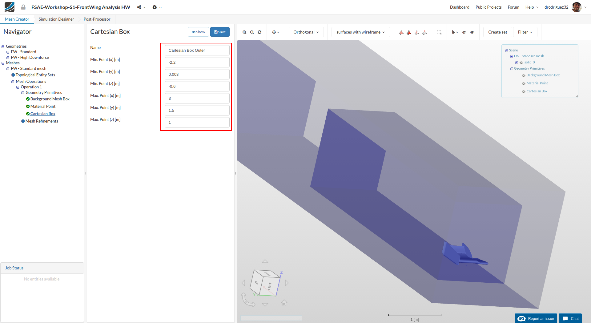
After creating a new Cartesian Box, you will be directed to the definition of this Cartesian Box. Change the dimensions of the box to the following:
- Min. Point (x) = -2.2
- Min. Point (y) = .003
- Min. Point (z) = -0.6
- Max. Point (x) = 3
- Max. Point (y) = 1.5
- Max. Point (z) = 1
Click Save to register your changes.
Cartesian Box - Inner
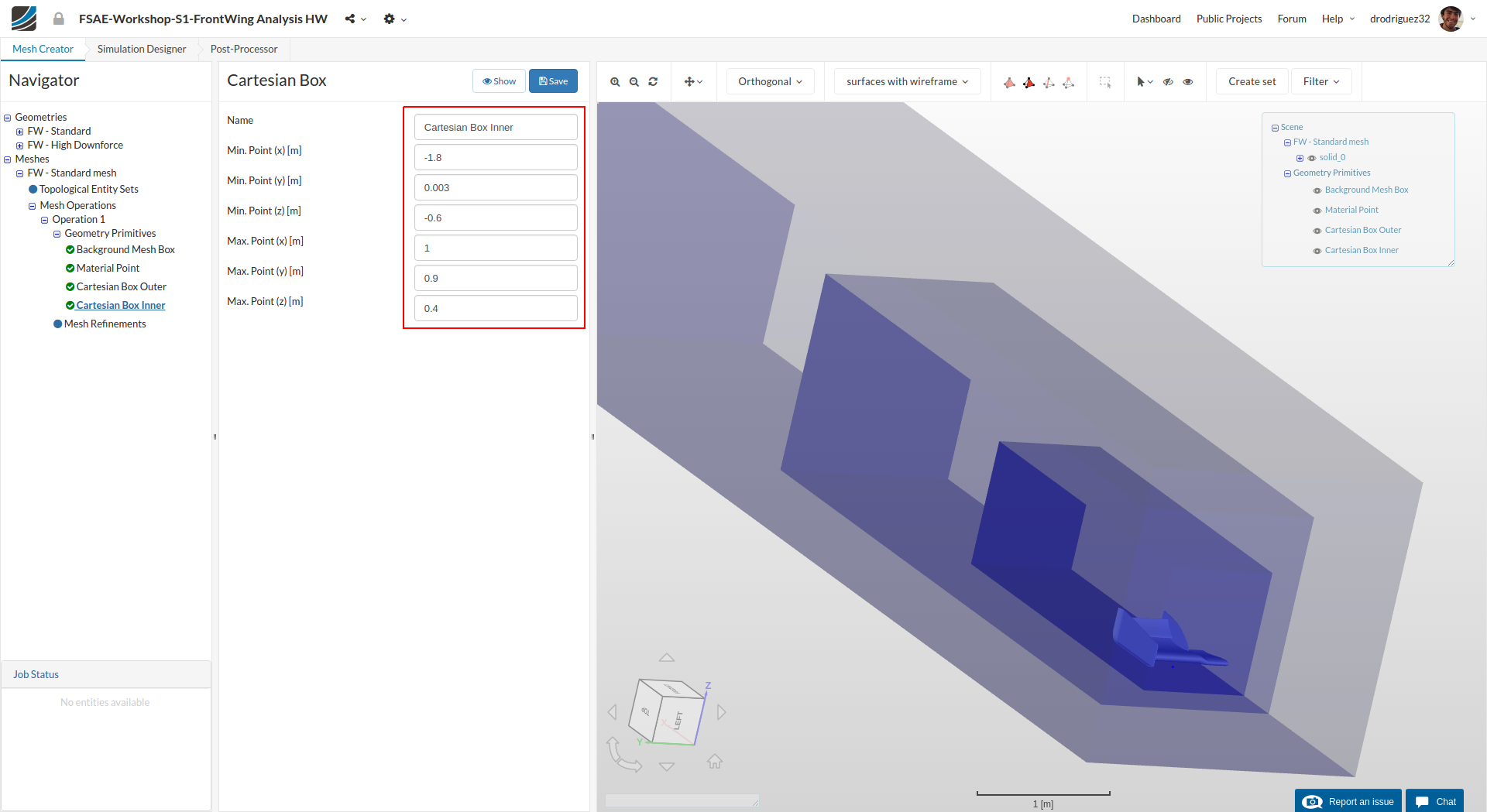
Follow the same procedure to define another Cartesian Box for further refinement definitions. Rename it to Cartesian Box Inner. This time change the values to the following:
- Min. Point (x) = - 1.8
- Min. Point (y) = .003
- Min. Point (z) = - 0.6
- Max. Point (x) = 1
- Max. Point (y) = 0.9
- Max. Point (z) = 0.4
Click Save to register your changes
With these Cartesian Boxes that we created we will define refinement regions where cells will be smaller and thus we will be able to observe more detail in the complex areas of the flow - a mesh that is too coarse will not allow you to observe small flow structures.
Mesh Refinements
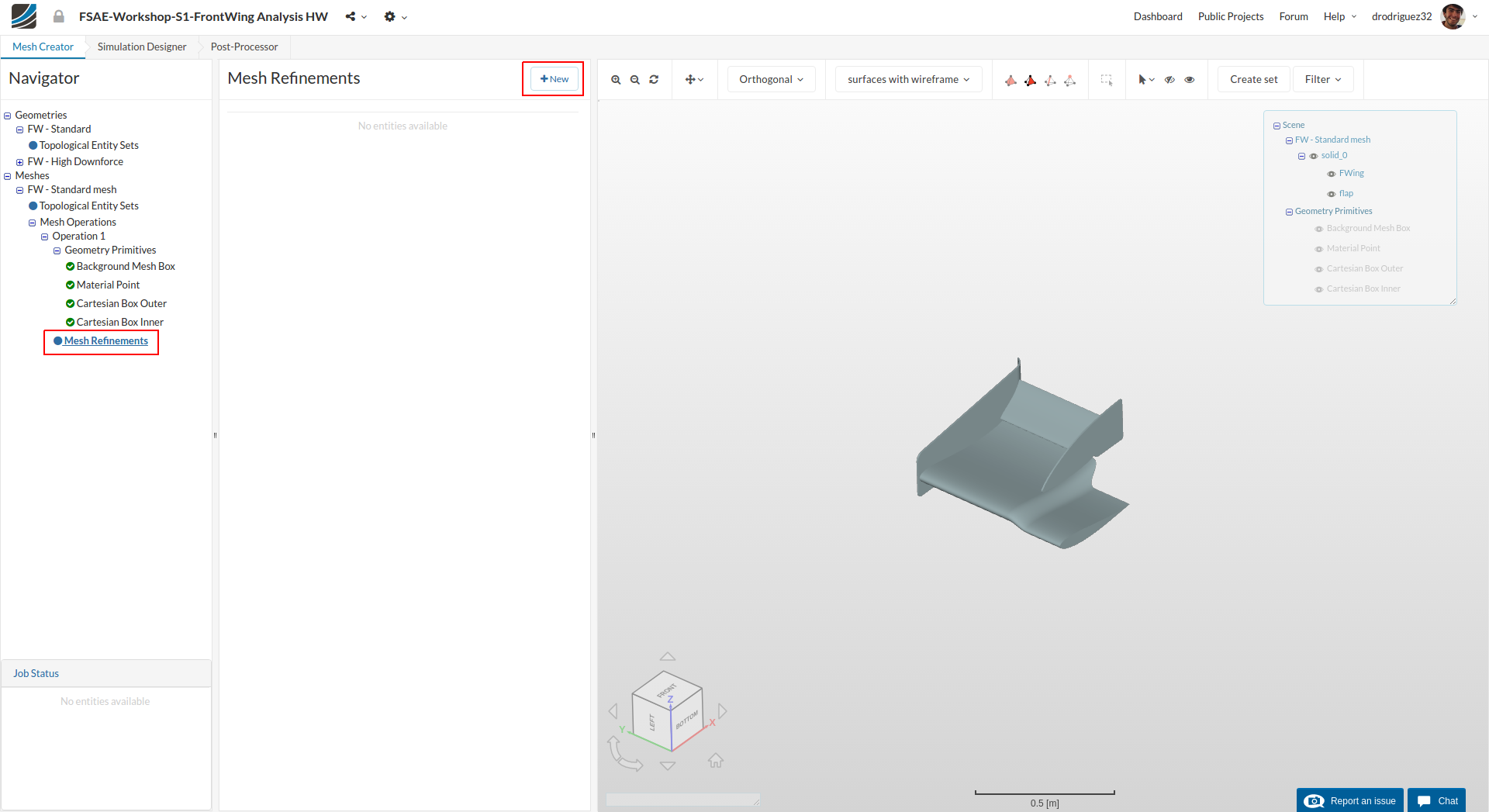
A good mesh requires well defined refinements. Now we will start creating the mesh refinements. For this proceed to Mesh Refinements and click +New
How does a mesh refinement work? It divides each cell to create more, smaller cells, and each level of refinement applies this to the cells generated in the past refinement level. This means that each cell that is refined will be divided into 4 smaller cells for each level. Example: at level zero you have 1 cell, at level one you have 4 cells, at level two you have 16 cells, at level three you have 64 cells, and at level four you will have 256 cells.
Mesh Refinement 1
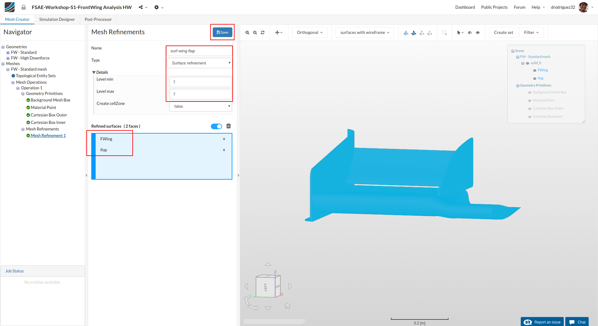
Rename it to surf-wing-flap (optional).
Change the Type to Surface refinement and then both Level min and Level max to 7 respectively.
Select the main wing and the flap - you should see that under Refined surfaces FWing and flap should be selected.
With this refinement we are improving the mesh that sits directly on the surface of the geometry. We do this to capture more accurately more details of the geometry and to better observe how the flow interacts with the surface of the wing.
Click Save to register your changes.
Mesh Refinement 2
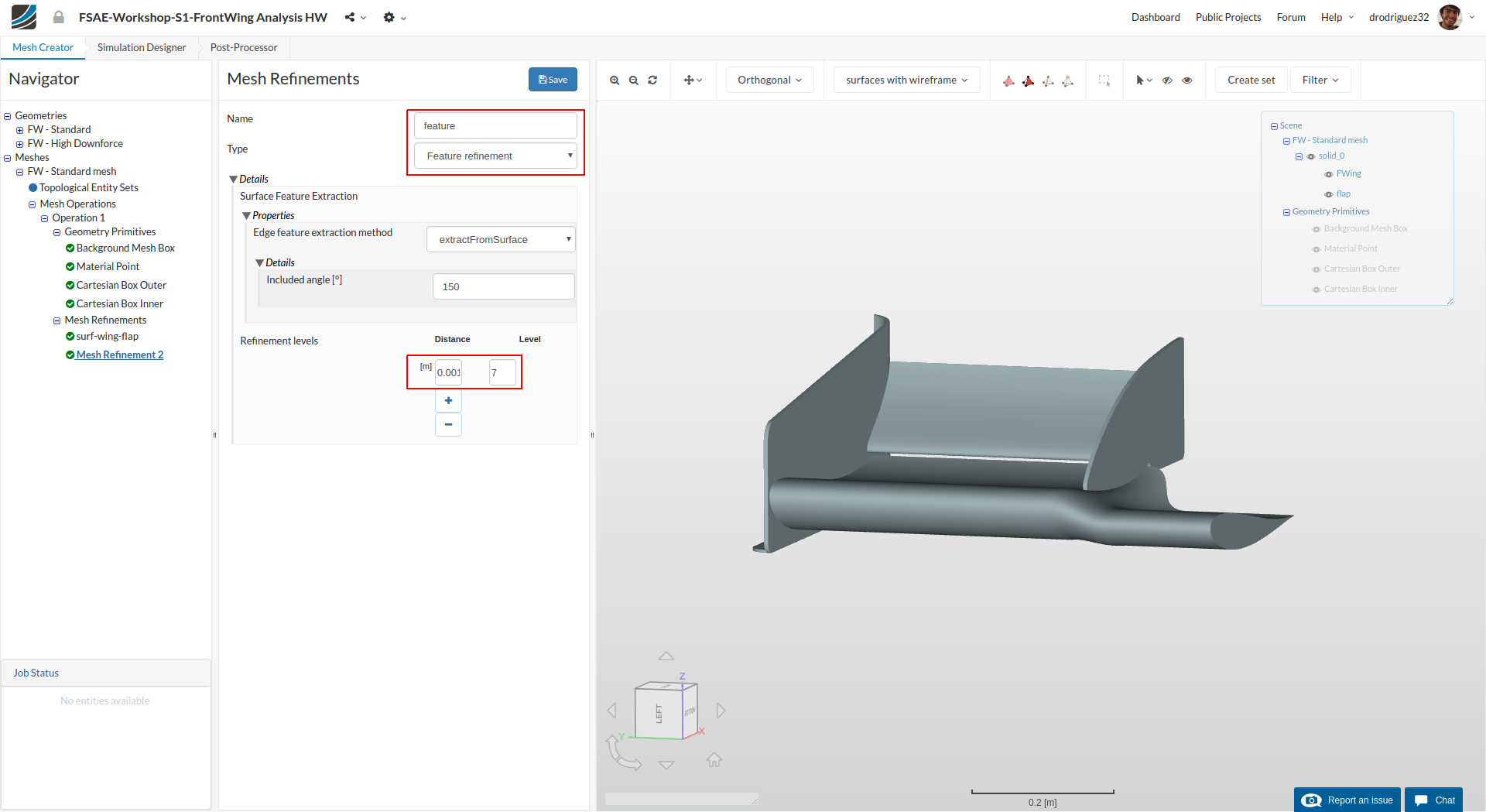
Following the same procedure, create a new refinement and name it feature (optional).
Under Refinement levels change Distance and Level to 0.001 and 7 respectively.
This refinement specifies that at a distance of 0.001 m from every edge and corner the mesh will be refined up to level 7. Again, this helps us capture the most complex features of the geometry and get better results around these areas.
Then click Save
Mesh Refinement 3

Now we will start refining the regions (Cartesian Boxes) that you created earlier.
Create a new refinement and rename it to region-inner (optional). This will be the smaller Cartesian Box.
Change Type to Region refinement and then under Refinement levels change Level to 3
Select Cartesian Box Inner under Geometry Primitves and click Save to register the refinements for this specific Cartesian box.
This is the region closest to the wing, so flow structures will be more complex immediately around and after the wing. So we want this area more refined.
Mesh Refinement 4
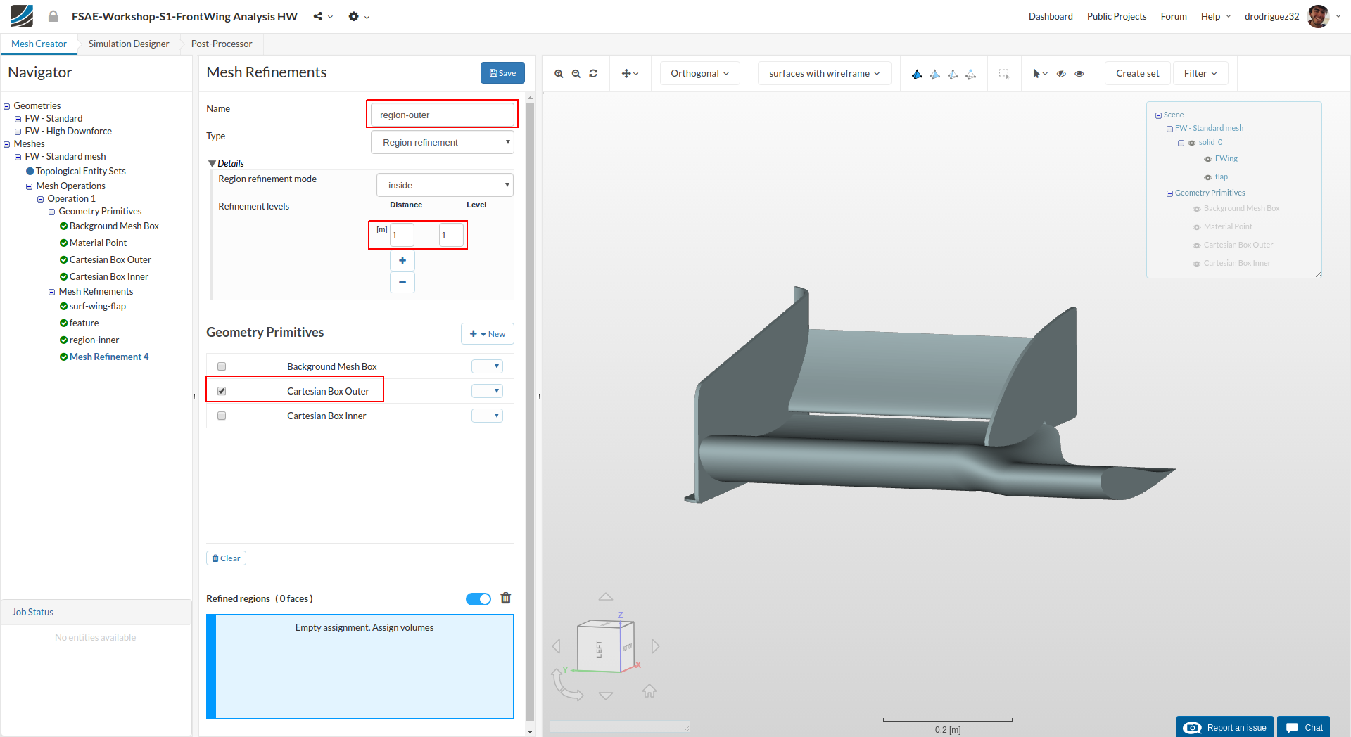
Create a new refinement for the other Cartesian Box. This time rename it to region-outer (optional).
Change Type to Region refinement and then under Refinement levels change Level to 1
Select Cartesian Box Outer under Geometry Primitves and click Save to register the refinements for this specific Cartesian box.
Further away from the wing we won’t have such complex flow, but because we are still considerably close and the flow is still affected we want this region slightly refined as well.
Mesh Refinement 5
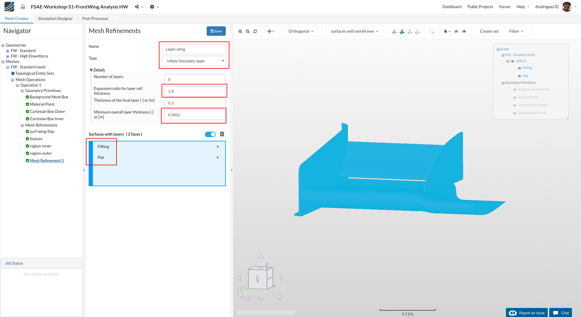
Next we will add layers over the surfaces on the whole wing and the floor. Layers will create small cells along every face of the geometry and allow us to capture the results near the surfaces (like the development of the boundary layer) more accurately.
Create a new refinement and rename it to Layer-wing (optional).
Change Type to Inflate boundary layer and then change Expansion ratio for layer cell thickness and Minimum overall layer thickness [-] to 1.8 and 0.0001 respectively.
The expansion ratio defines how fast the boundaries will grow - how much larger the next boundary cell will be compared to the past. And the minimum overall thickness defines a minimum limit to the size of the boundary layers - if the overall thickness is below this number, the algorithm will consider it not significant and no layers will be added.
Select the main wing and the flap. Under Surfaces with layers you should see FWing and flap are selected.
Click Save to register your changes.
Mesh Refinement 6
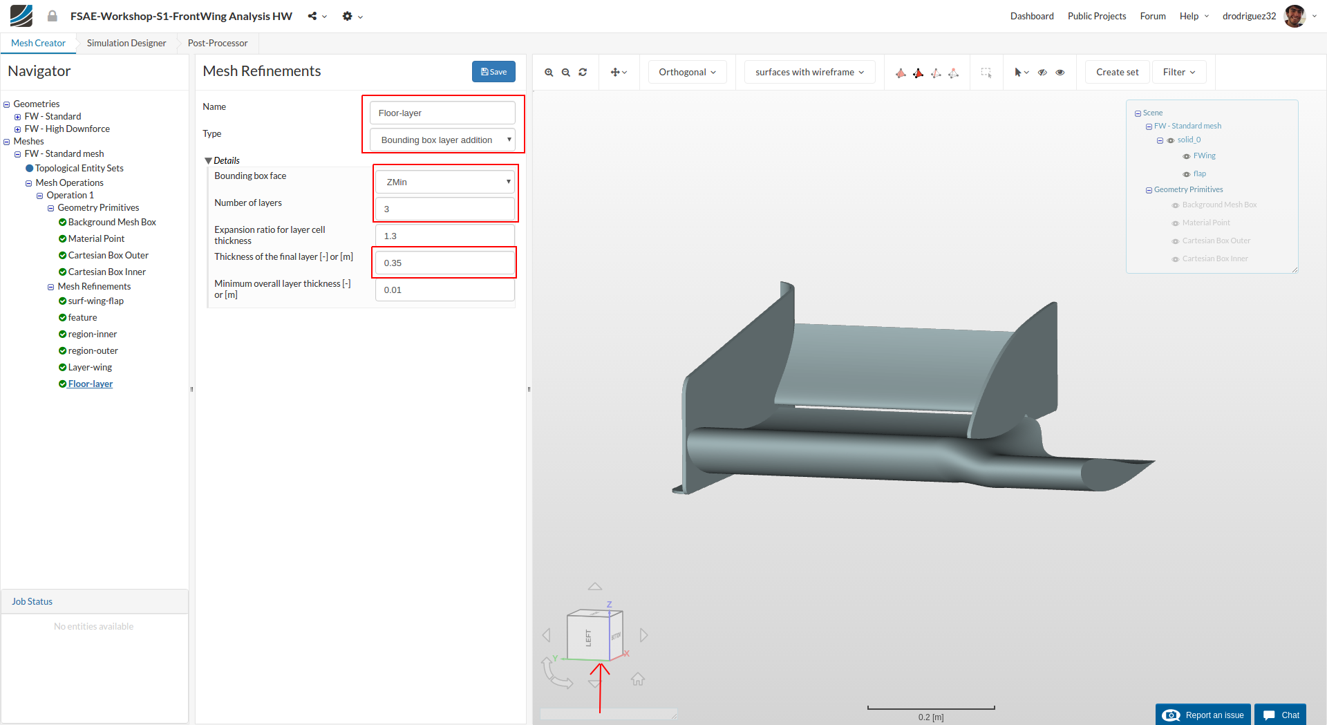
For the floor layers, create a new refinement and rename it to Floor-layer (optional).
Change Type to Boundary box layer addition
Change Bounding box face to Zmin and then the Number of layers and Thickness of the final layer [-] to 3 and 0.35 respectively.
Here we are creating boundary cells like in the past refinement, but these are applied to the floor.
Start Operation
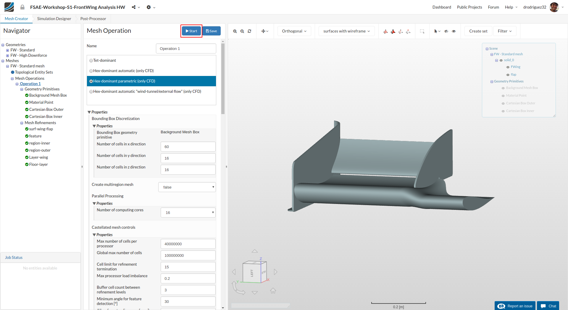
Once you have defined all of the mesh refinements, go back to the Operation 1 and click Start in order to submit the meshing job to the server. Due to the fineness of the mesh, the meshing could take around 30 minutes to finish. When the meshing is done you will see a green sign that says FINISHED when you click on your mesh.
Additional Meshes
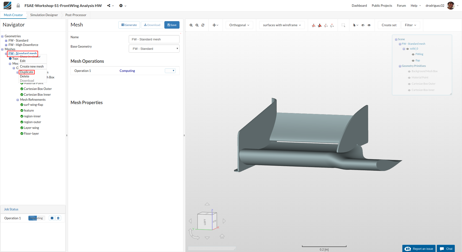
While the first mesh job is running, take advantage of parallel computing and proceed to start setting up the other configuration(s). You don’t have to perform all the meshing operations again from scratch. Just duplicate the already created mesh by right clicking on it and then click Duplicate.
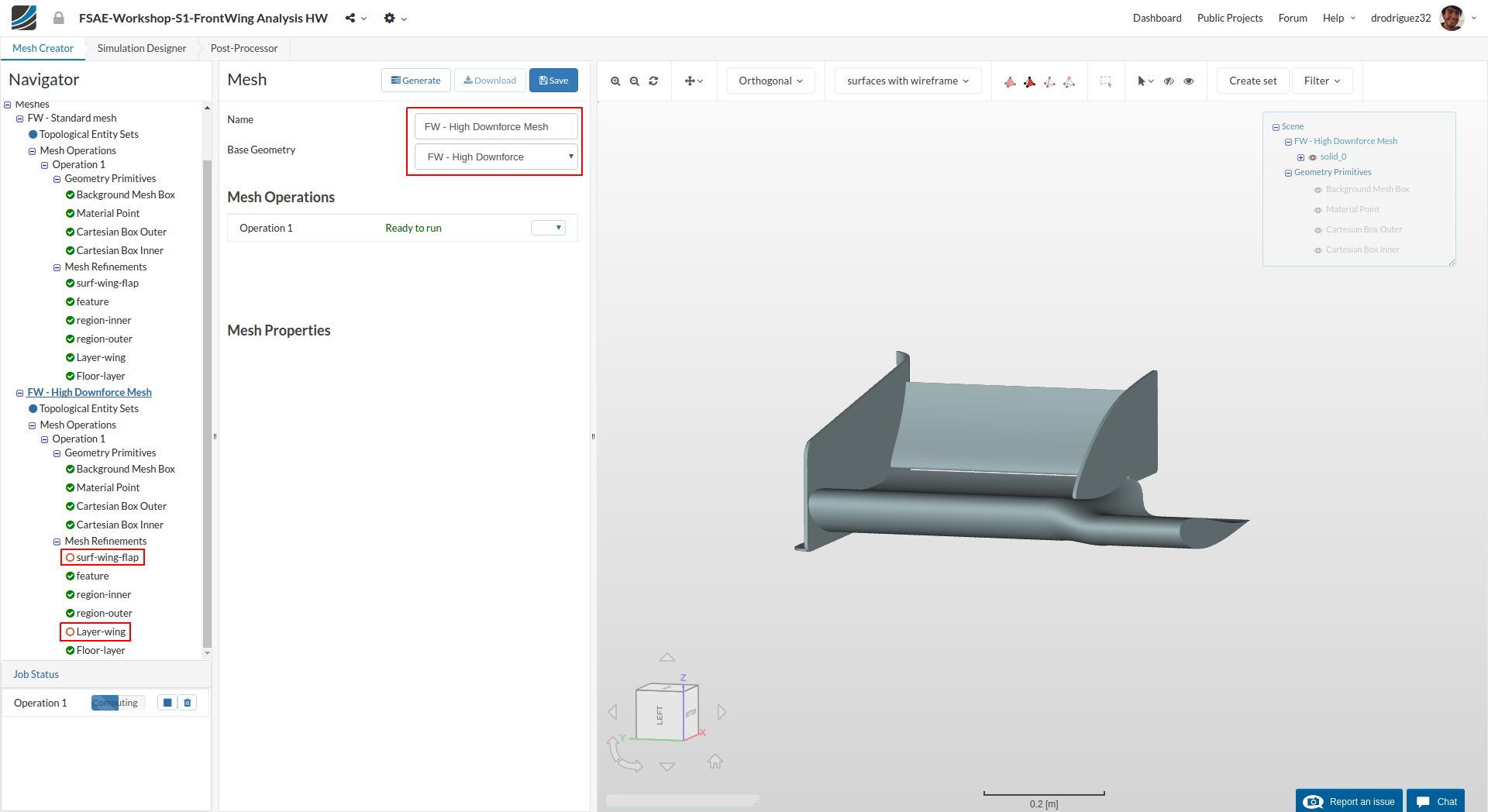
Rename the duplicated mesh and use the drop-down to change the Base Geometry to the model other model. Then click Save. Now you will have to reassign the Fwing and flap faces for surf-wing-flap and Layer-wing refinements and start the meshing operation.
Mesh Quality
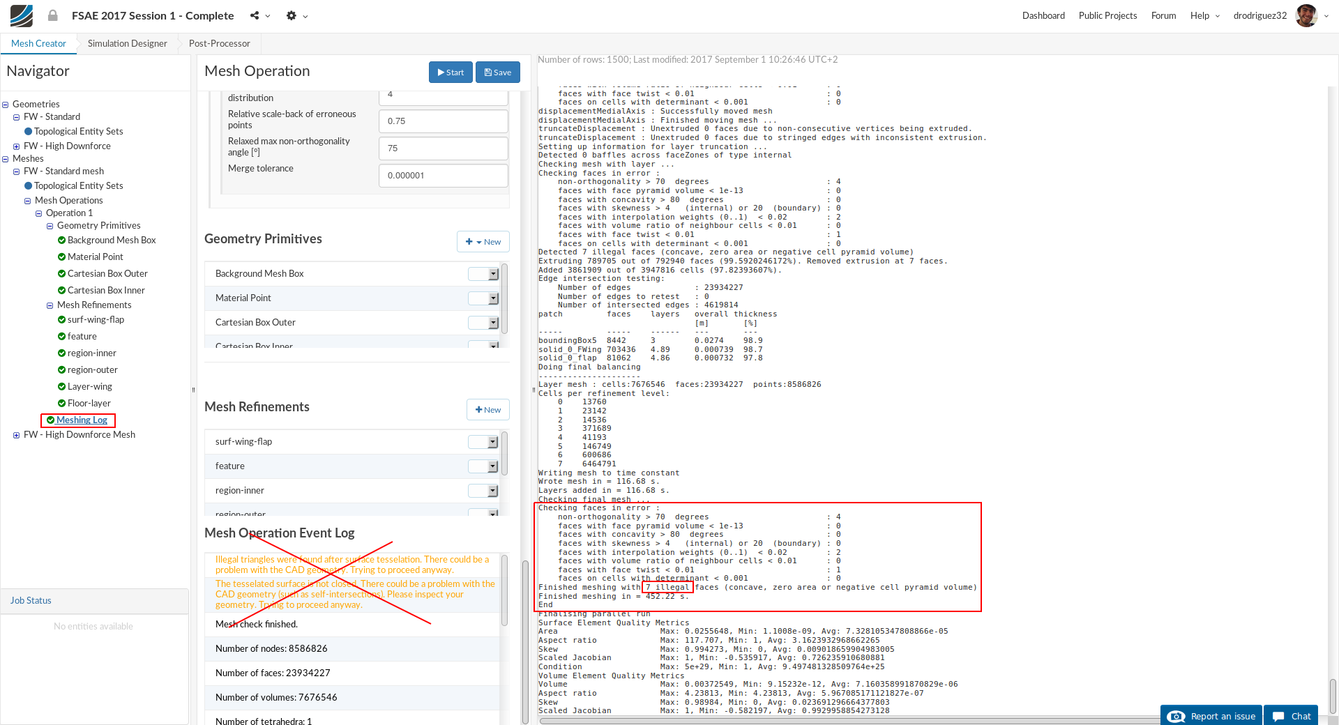
When your meshing process is done, don’t look at the Mesh Operation Event Log. If you want to check the quality of your mesh please click on Meshing Log in the Navigator and scroll to the bottom of the text log. There should be around 7 illegal faces (like in the picture) - don’t worry, as long as the number of illegal cells is close to the picture, your simulation will run.
Simulation Setup
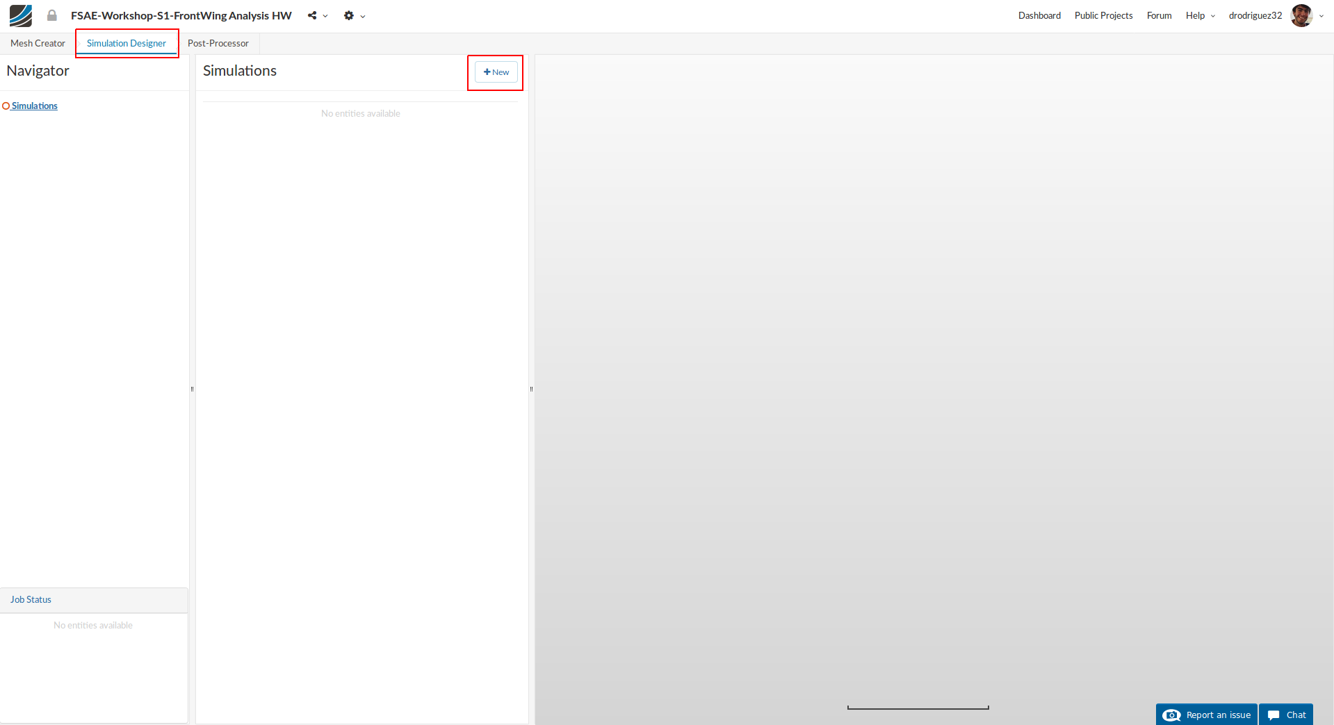
Once the meshing of the first geometry is finished, you can proceed to Simulation Designer without waiting for others to complete in order to set up the simulation in parallel.
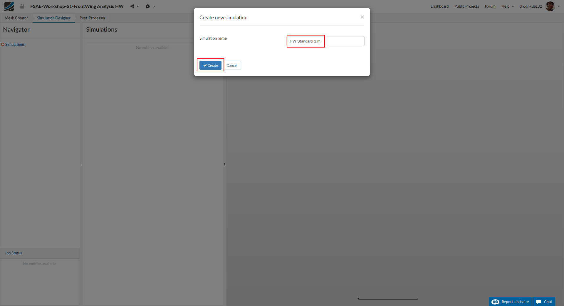
Once you are in Simulation Designer, click New Simulation in order to start setting up the simulation. A new simulation creating window will pop up. Rename it to FW Standard Sim (optional) and click Create in order to create a new simulation.
Analysis type
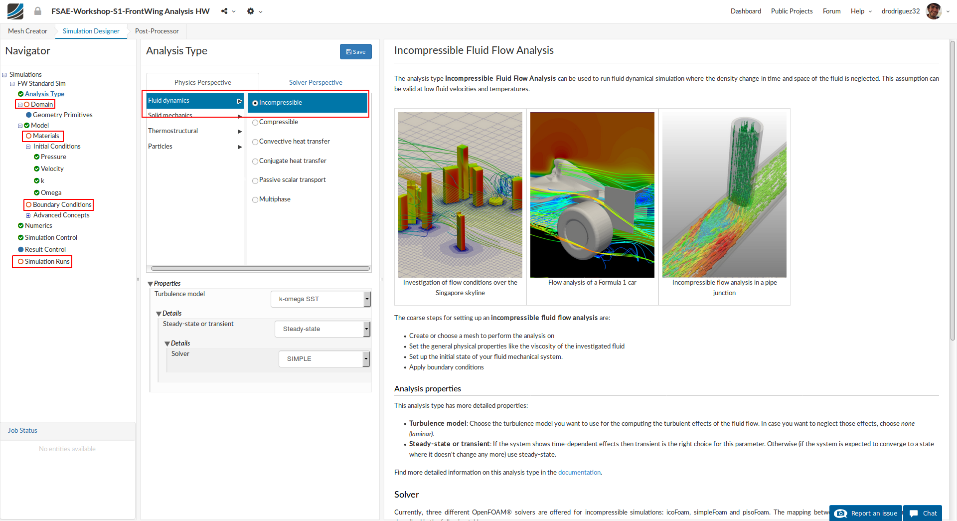
In Analysis Type, switch to Fluid dynamics and then select Incompressible. You don’t have to change any properties here.
Click Save to select this analysis type.
Once you save the analysis type, you will see the expanded navigator tree. All the red entities shows that they must be set up in order to perform a successful simulation run.
Domain
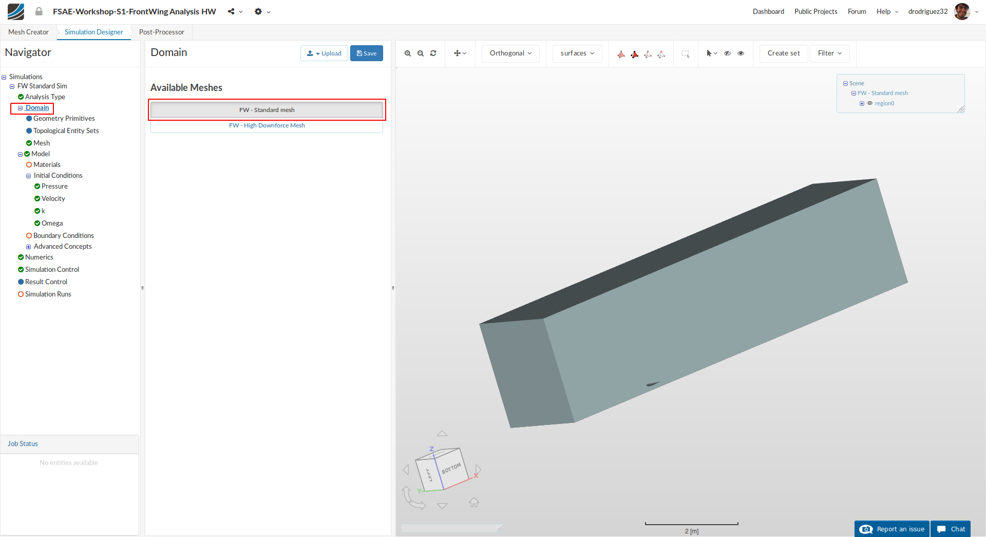
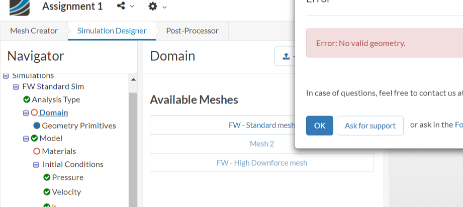
Next you have to select a domain on which this simulation will be performed. Proceed to Domain and select FW-Standard-Mesh and click Save.
After a while you will see the loaded mesh of the selected domain in the viewer. For the easier mesh handling, it is recommended to switch to the surfaces render mode in the top viewer bar.
Material
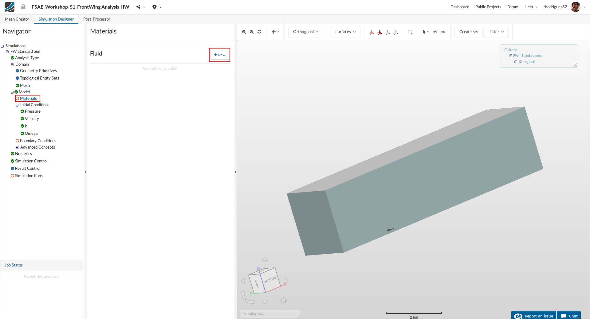
Next we have to define the fluid material. Go to Materials and click on +New to create a new material.
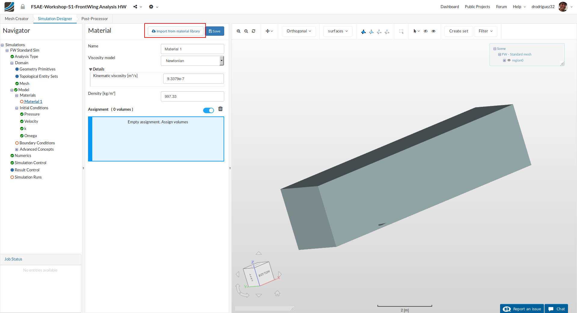
Click on Import from material library to import the desired material from the material database.
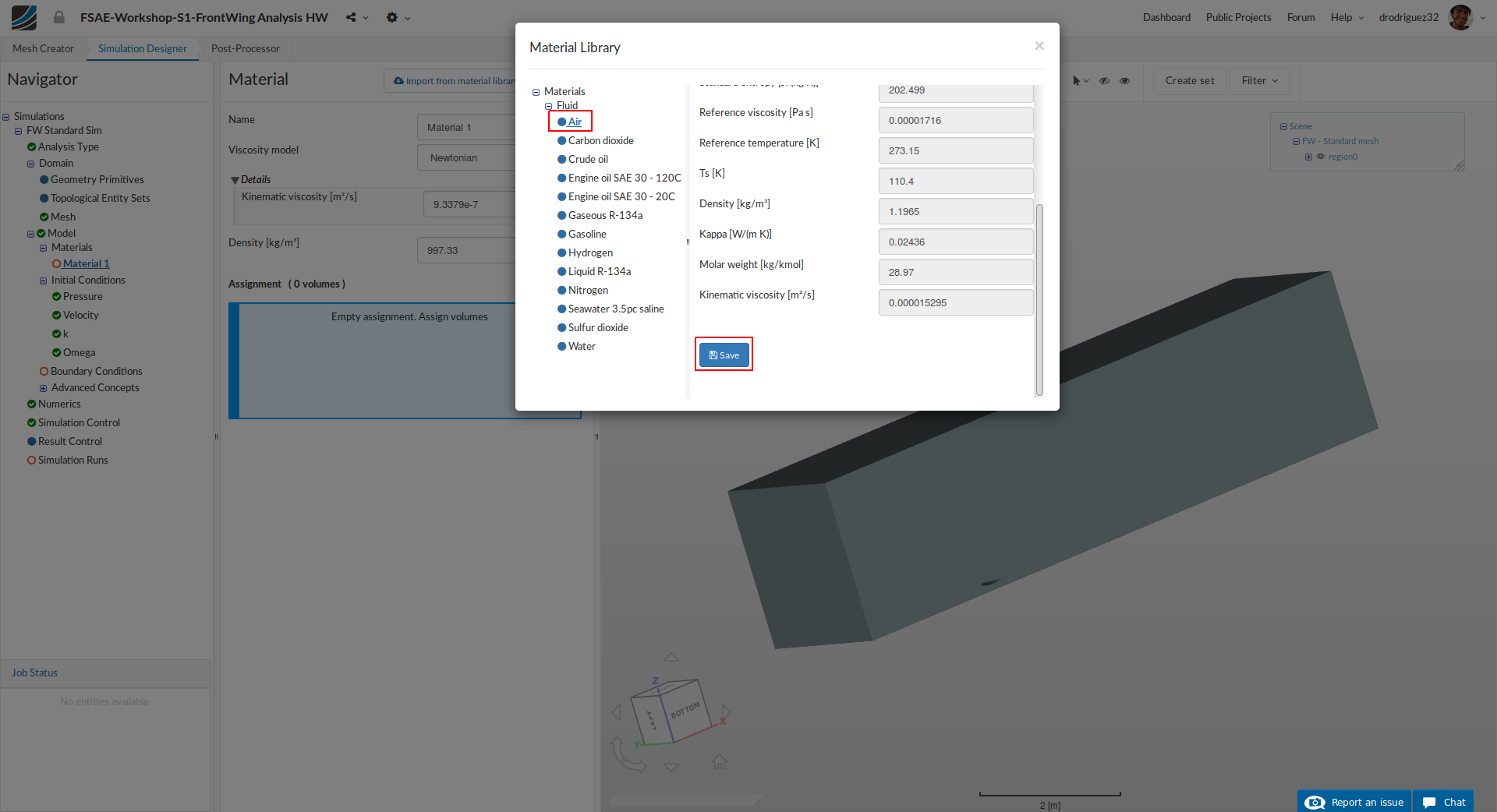
Select Air and click Save to import this material directly from the library.
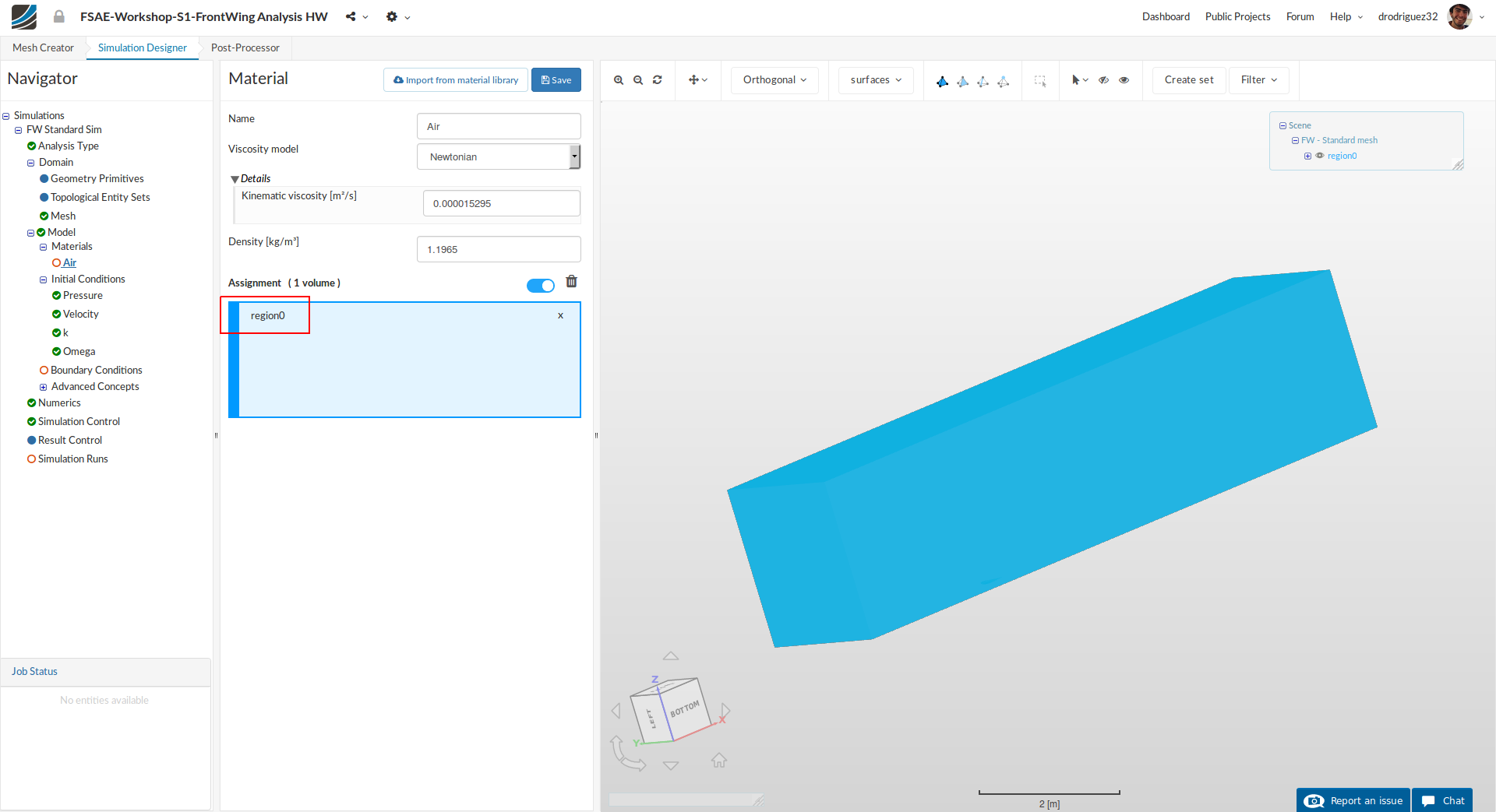
Select region0 under Assignment and then click Save in order to define the material for this region.
Initial Conditions
Pressure and velocity we will leave as the default set by SimScale.

Go to k and change the Turbulent kinetic energy value [m²/s²] value to 0.24 and click Save
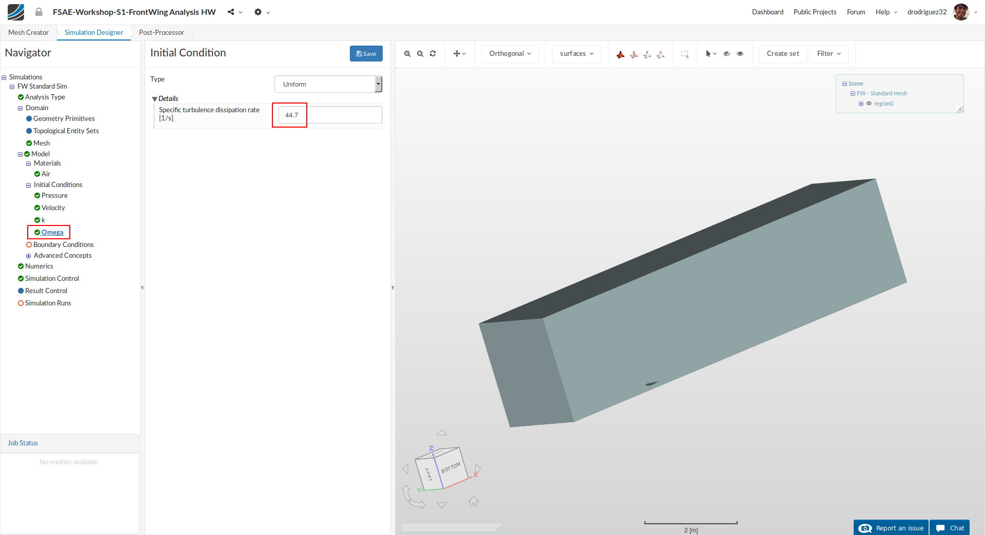
Next go to Omega and change Specific turbulence dissipation rate [1/s] to 44.7 and click Save
The two settings you just modified are associated to the turbulence model that will be applied to this simulation (K-Omega SST). Turbulence is a highly complex process with irregular, chaotic, and unsteady 3D phenomenon. We would need an extremely fine mesh and a huge amount of computational power to correctly simulate it, so the standard process is to apply a model that mathematically predicts this turbulent behavior.
Boundary Conditions
This is one of the most important parts of the simulation set-up. Boundary conditions are how we tell the platform how each thing behaves. So for example where does the air go in and where does it go out? With what speed does the air go into the domain and in what direction? Is the air being slowed down by something (like the wing)? This is what you’ll do now.
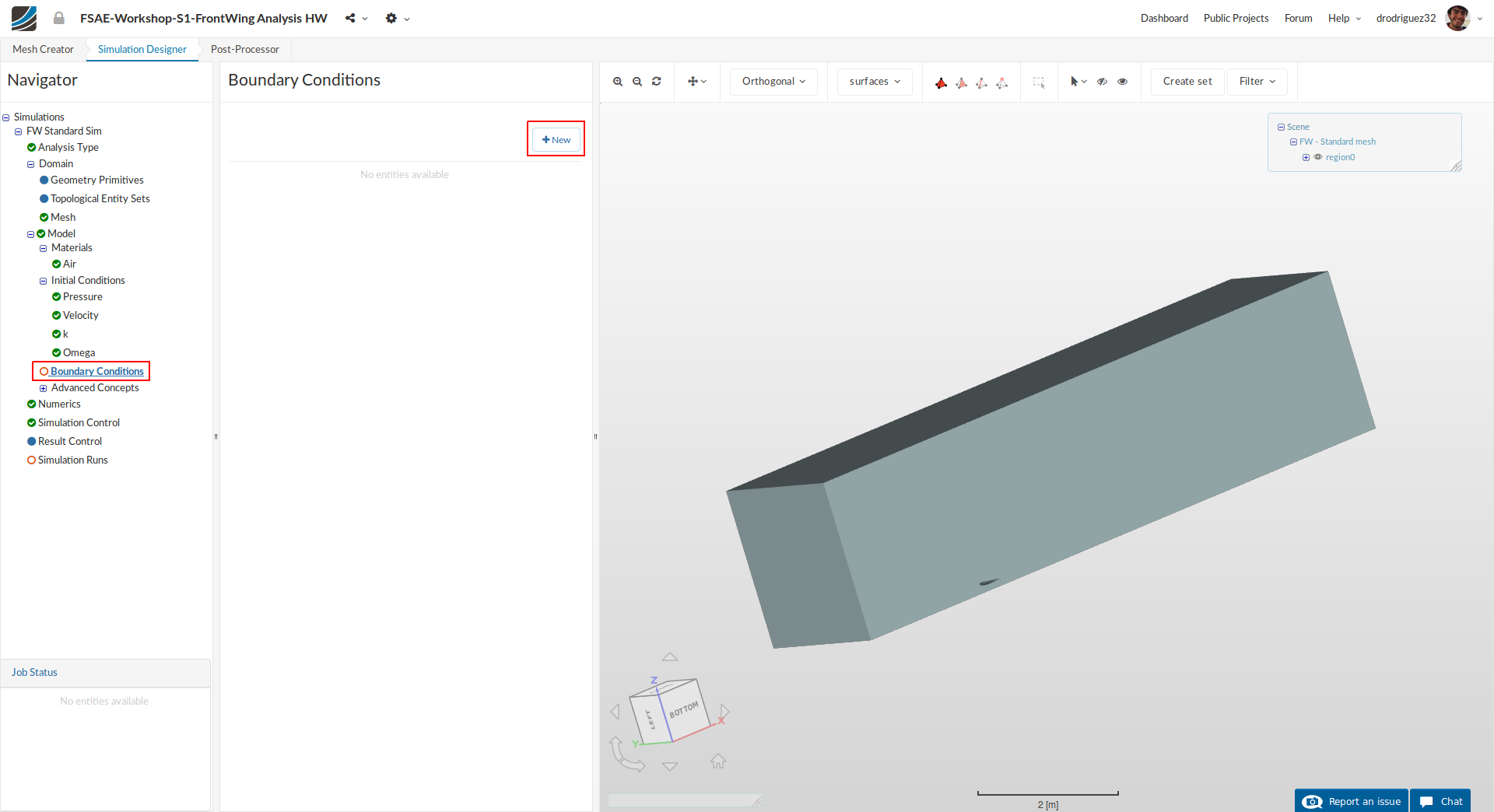
Go to Boundary Conditions and click +New in order to create a new boundary condition.
1. Inlet
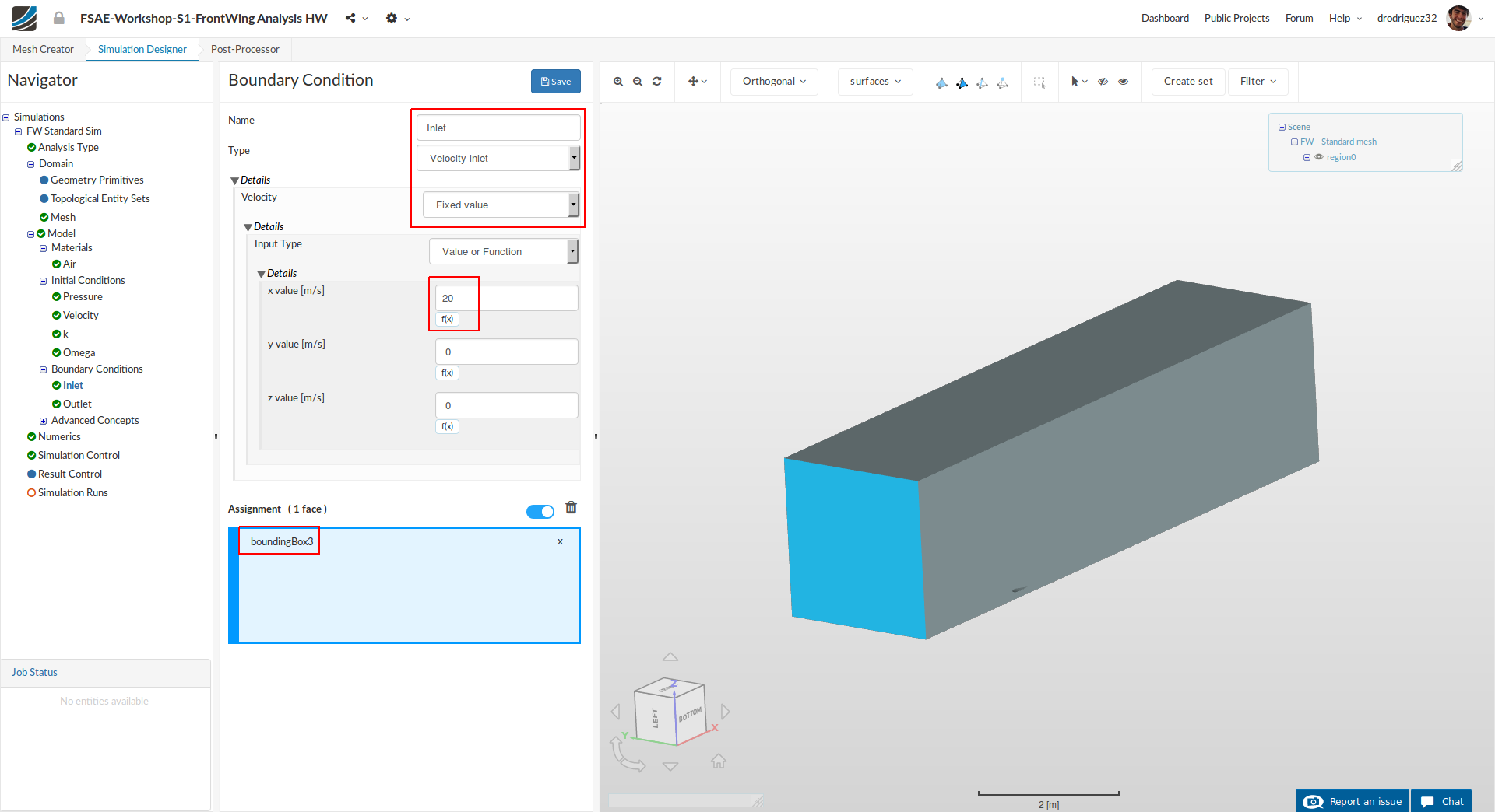
Rename the newly created boundary condition to Inlet (optional).
Make sure that the Type is Velocity Inlet and that under Velocity it says Fixed value. Change the x value [m/s] to 20
Select the front surface of the domain from the viewer and under Assignment you should see boundingBox3.
Click Save to define the inlet boundary condition.
2. Outlet
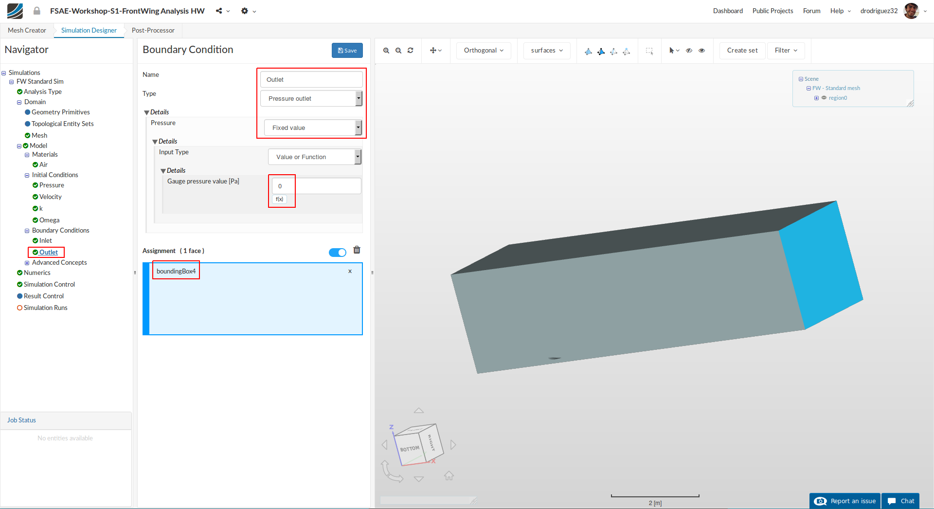
Create a new Boundary Condition and name it Outlet (optional).
Change Type to Pressure Outlet and select the back surface of the domain. Under Assignment you should see boundingBox4.
Click Save to define the outlet boundary condition.
3. Sides
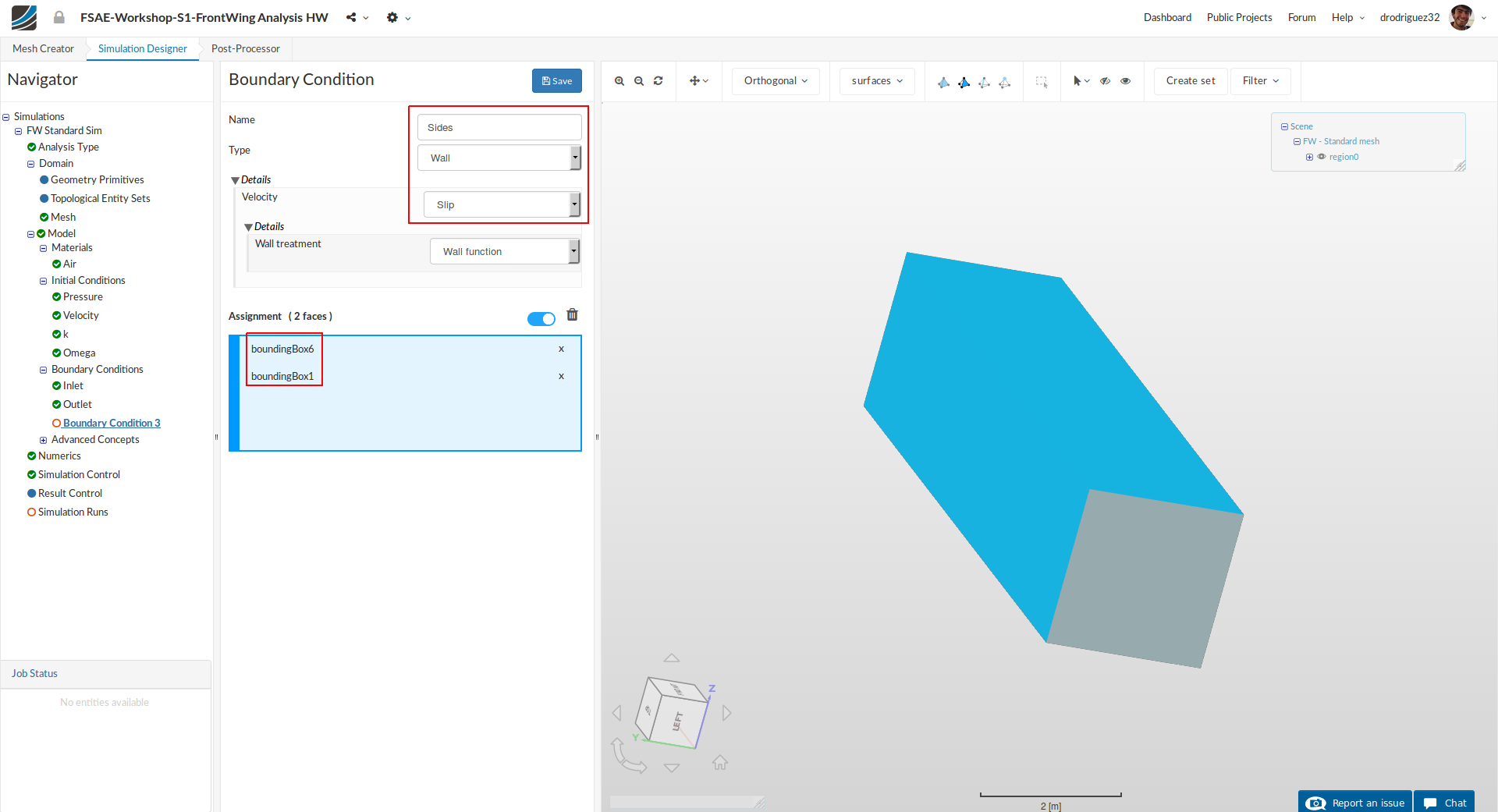
Create a new Boundary Condition and name it Sides (optional).
Change Type to Wall and Velocity to Slip.
Select the side face (away from the wing) and the top face of the bounding box. Under Assignment you should see boundingBox6 and boundingBox1.
Click Save to define the boundary condition for the sides.
4. Symmetry
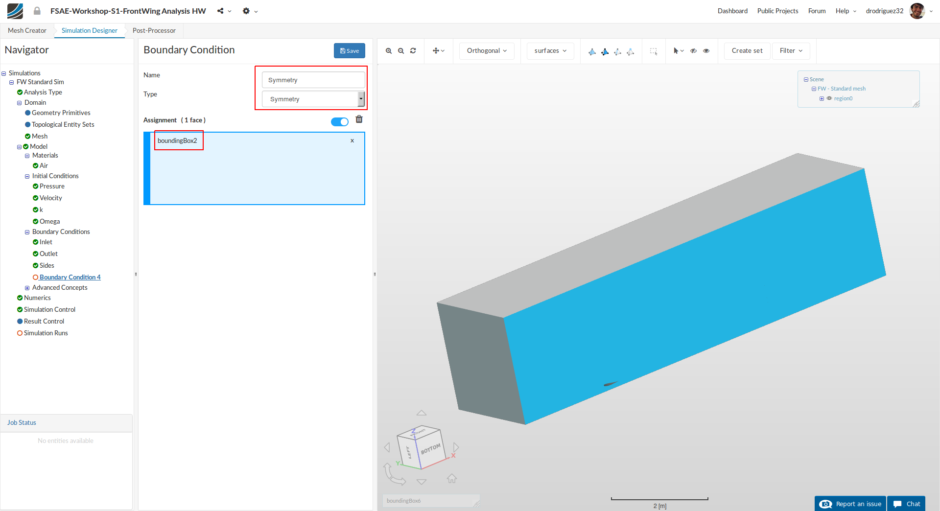
Next we will define the symmetry condition. This is what tells the simulation that in reality we are running a complete wing. Create a new Boundary Condition and name it Symmetry (optional).
Change Type to Symmetry and select the side face on the inner side of the wing (where it was cut) (boundingBox2).
Click Save to define the symmetry boundary condition.
5. Floor
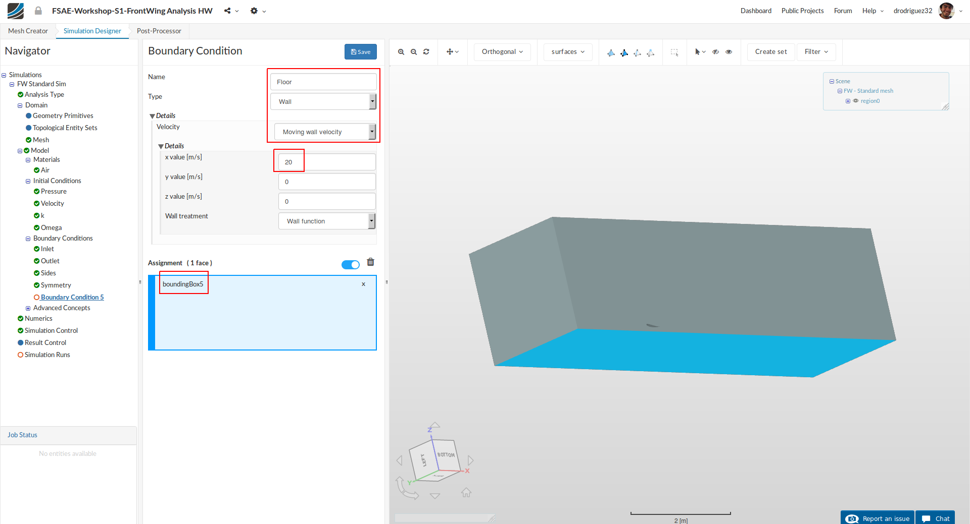
Create a new boundary condition and rename it to Floor (optional).
Change Type to Wall and under Velocity select Moving wall velocity. Change the x value [m/s] to 20. With this you’re now saying that the floor also moves past the car (maintaining the condition that there is relative motion between the car and the floor and there isn’t relative motion between the air and the floor.
Select the floor of the bounding box domain and under Assignment you should see boundingBox5.
Click Save to define the floor boundary condition.
6. Wing
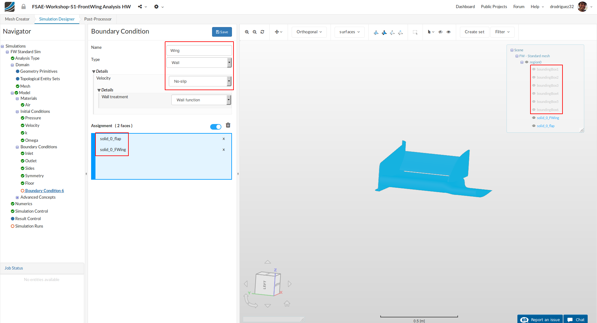
Finally, we will define the boundary condition for the wing. Create a new boundary condition and rename it to Wing (optional).
Change Type to Wall and Velocity to No-slip. Also, make sure under Wall treatment it says Wall function.
With this No-slip condition you are specifying that there is friction between the car and the air and thus a boundary layer will be formed.
Make sure you hide the bounding box by using the navigator on the right. Select all the wing.
Click Save to define the boundary condition for the wing.
Numerics
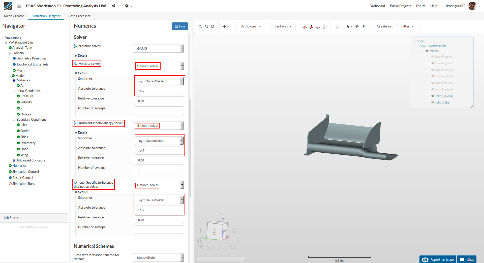
After defining all the boundary conditions, we will proceed to set up the numerics for our simulation. Go to Numerics and scroll down until you reach Solver.
Under Solver, change [U] velocity solver to Smooth solver. Expand Details and change Smoother to symGaussSeidel and Absolute tolerance to 1e-7.
Do similar changes for [k] Turbulent kinetic energy solver and [omega] Specific turbulence dissipation solver.
Click Save to register your changes.
Simulation Control
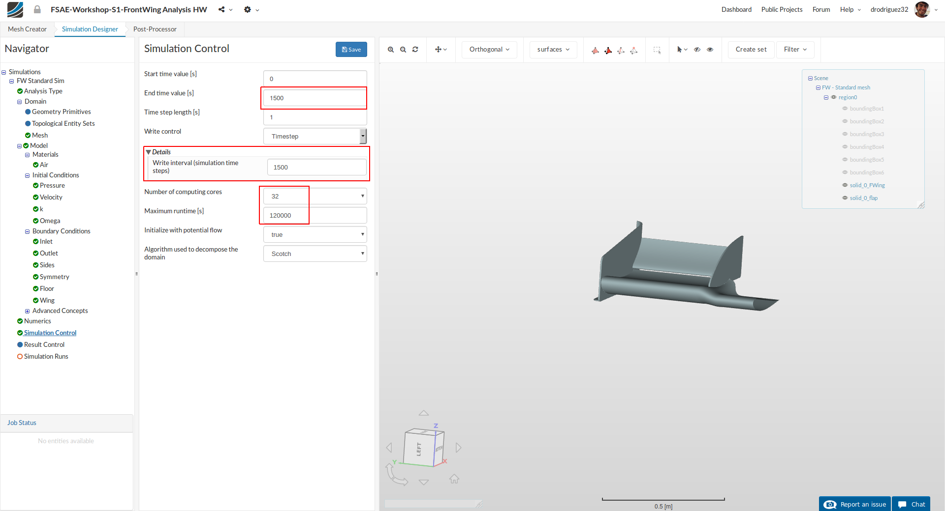
Next we will define the our simulation interval and steps that needs to be recorded. Go to Simulation Control and change End time value [s] to 1500.
Expand Details under Write control and change Write interval (simulation time steps) to 1500.
Next change Number of computing cores and Maximum runtime [s] to 32 and 120,000 respectively. The Maximum runtime [s] is set too high just to be on a safe side, because if the simulation runs for longer than that time it is cancelled.
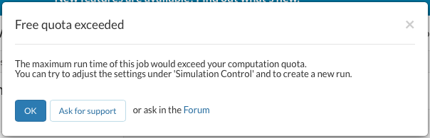
If you are on the Professional Account Trial the setting for Maximum Runtime will be too high for the simulation to run. You can change it to 12,000 s or contact us so that we can change your account to a free community plan.
Please take not that if you are on the Professional Account Trial you will not be able to through all the workshop sessions, so it is recommended to change your account to the Community Plan. You can do this by contacting us directly.
Click Save to register your changes.
Result Control
As our last step before running the simulation, we will create result control items in order to get graphical data sets of interest. These control items allow us to see when a simulation has reached steady state (when forces become constant) and it also lets us see things like the lift and drag of the wing.

Go to Result Control in the navigator. We will create the result control item for the forces and moments. Click New next to Forces and Moments.
1. Main Wing
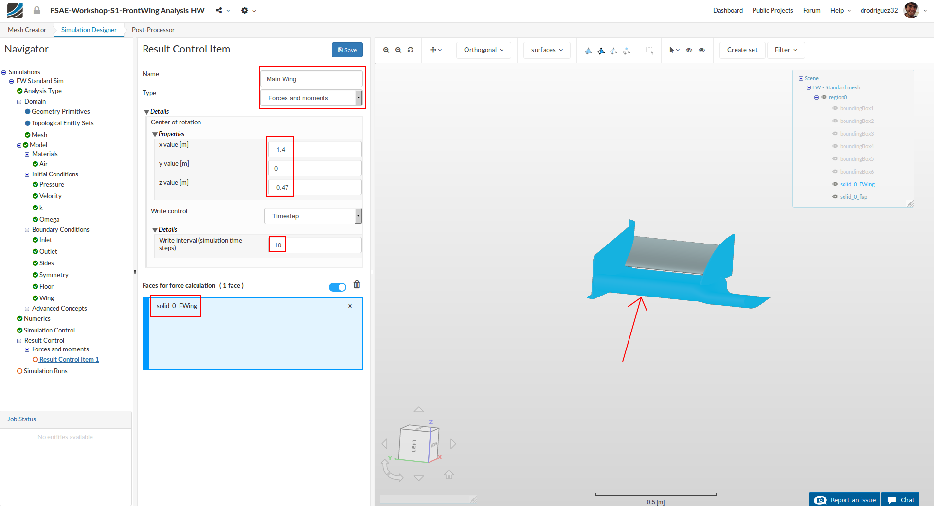
A new force and moment result control item will be created. Rename it to Wing main (optional).
Then change x value [m] to -1.4, z value [m] to -0.47, and Write interval (simulation time steps) to 10.
Select the main wing and under Faces for force calculation you should see FWing.
2. Flap
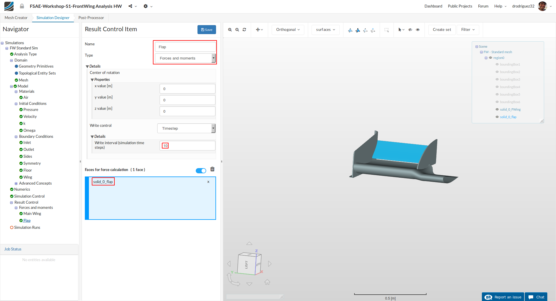
Create another force and moment result control item and rename it to Flap (optional). Change the same values as defined above but this time select the flap and you should see Flap under Faces for force calculation.
Click Save to save your changes.
3. Field Calculations
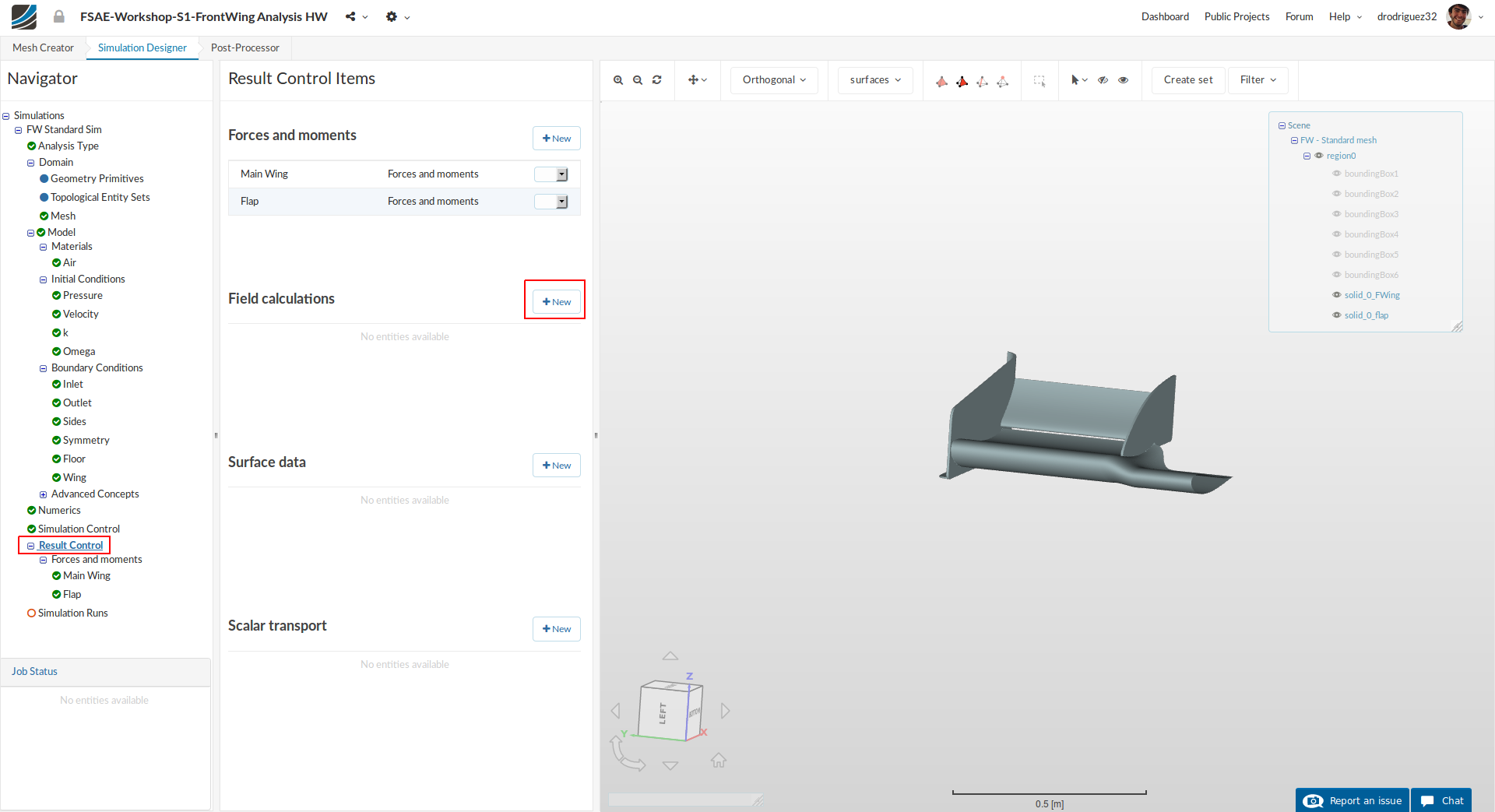
Next, we will create the field calculation items. For this go back to Result Control and click New next to Field calculations.
Y-Plus
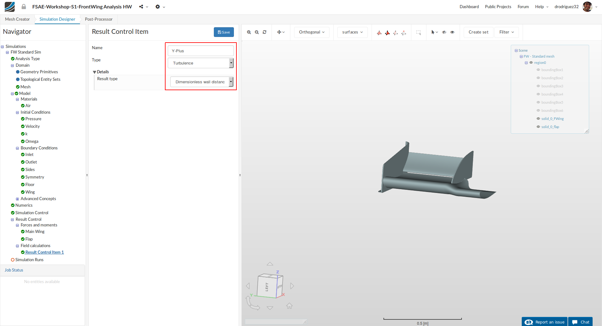
Rename the newly created field calculation item to Yplus (optional).
Change the Type to Turbulence and click Save to register your changes.
Wall Shear Stress

Create another field calculation item and rename it to WallShearStress (optional).
Change the Type to Wall fluxes and click Save to register your changes.
Simulation Runs
Once all the above steps are defined, we will proceed to create our first simulation run.
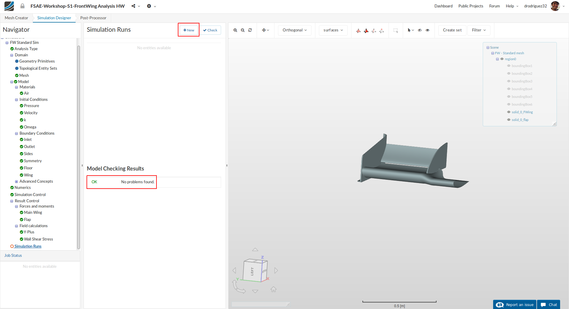
Go to Simulation Runs and click on New.
A window will pop up, give a reasonable name to the run e.g. Run-Standard in this case (optional) and click Start to initialize this run. The simulation run can take up to ~180 minutes (~3 hrs.).
Additional Simulation Runs
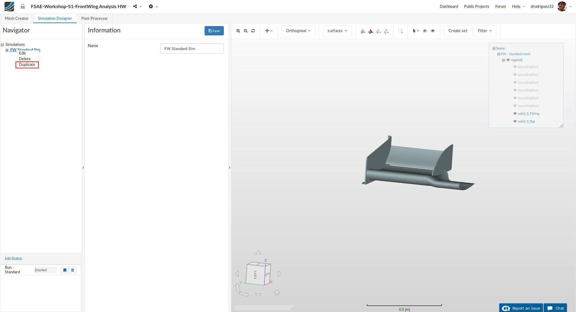
While the first simulation job is running, take advantage of parallel computing and proceed to start setting up all the other configuration(s). You don’t have to perform all the simulation set up operations again from scratch. Just duplicate the already created simulation by right clicking on it and then click Duplicate.
Rename the duplicated simulation to FW-High Donwforce-Sim and assign your new domain to the duplicated simulation under Domain.
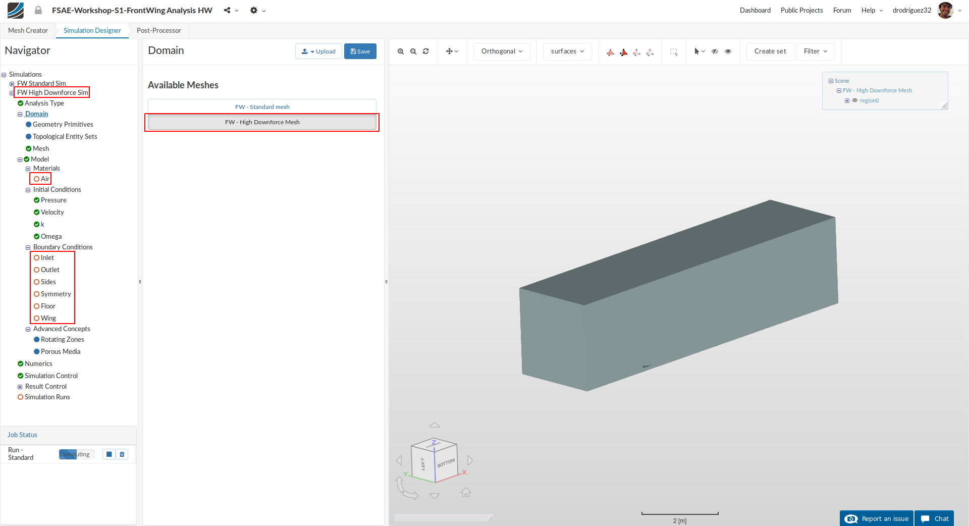
Then click Save. Now you have to just assign back all the entities to the material, boundary conditions and result control force plot items and then start the simulation job.
Recommendations About Comments
If you run into issues during your process, before adding a comment to the thread please consider the following:
- Go over the tutorial one last time and compare it to your setup. Is everything the same?
- Go over the existing comments. Maybe someone has had the same problem and it’s already solved.
- Is there an actual error? Or is it taking a long time to load?
a. If it seems to be a loading issue, please give it some time or refresh the page. Sometimes due to the internet connection the platform may seem slow.
If it’s a new issue that you can’t solve, please outline the issue as specifically as possible and include a link to your project. This will help us figure out what is going on faster and thus we can get back to you faster.
Continue to part 2 of the tutorial:
Step-by-Step Tutorial Session 1 - Front Wing Design Study (Part 2)