Dear Sir/Madam
I am conducting an indoor contamination test. The cylindrical objects in the model represent virtual sources of contamination. However, upon reviewing the Solution Fields, it seems that something may not be correct. I’m not sure if there is an error in the settings under Advanced Concepts or in the Solution Fields settings. Could you please assist me in making adjustments?
This is the workbench link of my work:
My research involves validating and comparing the diffusion of contaminants (such as Covid particles) in indoor spaces using SimScale.
I referenced the Car Park Contamination Simulation tutorial (Car Park Contamination Simulation Tutorial | SimScale) for my room contamination test, so I expect my results and visualization to be similar to Figures 26 and 27.
Regarding the parameter settings, I have a couple of questions:
In my room contamination test simulation, the cylindrical bodies represent the non-physical contamination zones. So, I wonder if my setup of momentum sources and passive scalar sources is correct?
In the tutorial, for the Iso Volume in Solution fields, how do I determine the appropriate minimum and maximum Iso value settings?
I believe that the contamination source (the cylindrical bodies) should appear as the most intense source of contamination, indicated by the highest passive scalar values. Additionally, the contaminated gas or particles should be directed towards the outlet positions (perhaps similar to the attached image?).
Hi @eaglechen thanks a lot for posting at our forum
I’d first like to say that your project sounds very interesting and I really enjoyed taking a closer look at it.
Regarding the answer to your questions,
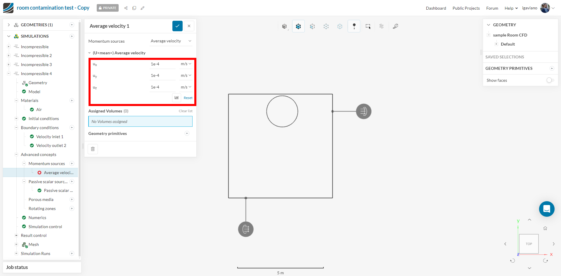
In the kind of simulation you’re trying to run, there seems to be no need for momentum sources since I assume the contamination would spread evenly accross the cylinder’s surface. However, the defined velocity should not be impactful in your case since it’s a very low value:
As to the passive scalar source, it seems fine. You can think of it as a concentration so that it’s value depends on which kind of unit you’re working with. Try thinking of it as ppm. More information can be found here.
The minimum/maximum iso value settings depends on which data you want to see. Perhaps there’s confusion regarding the expected results for that case, I’ll comment on that next.
Regarding the picture:
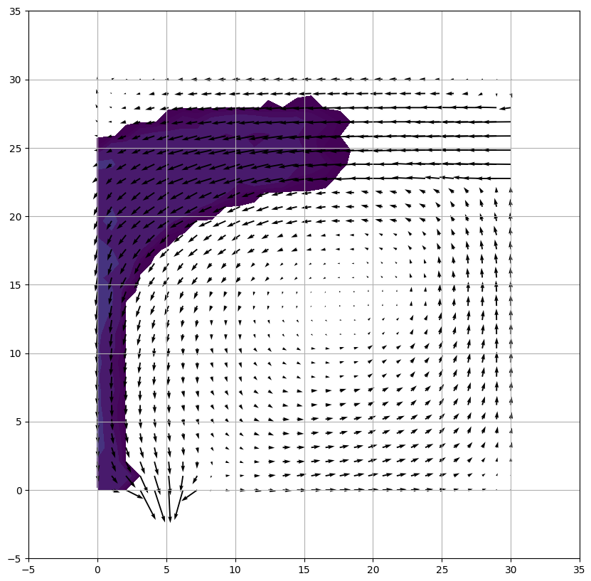
Is that simulation in the picture a transient one? I ask that because we should see the passive scalar dissipate to these regions given enough time due to advection, diffusion and turbulence:
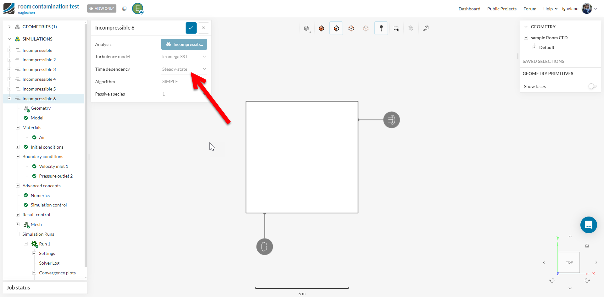
Since yours is a steady state simulation, why not trying to run a transient analysis instead and take a look at the results?
One last comment:
I see that you stablished a velocity boundary condition for both the inlet/outlet. While this is fine from a physics point of view, maybe changing the outlet to a pressure boundary condition (0 gauge pressure) would help the simulation provide better results. This OpenFOAM documentation provides useful combinations of inlet/outlet boundary conditions and their stability.
I’d like to ask you and discuss the following points:
Regarding the response about the image, could you please clarify what you mean by “transient one”? Does it mean that the wind field is fixed? About this image, I actually extended Ladybug from Rhino Grasshopper, which calculates a fixed wind field using OpenFoam.
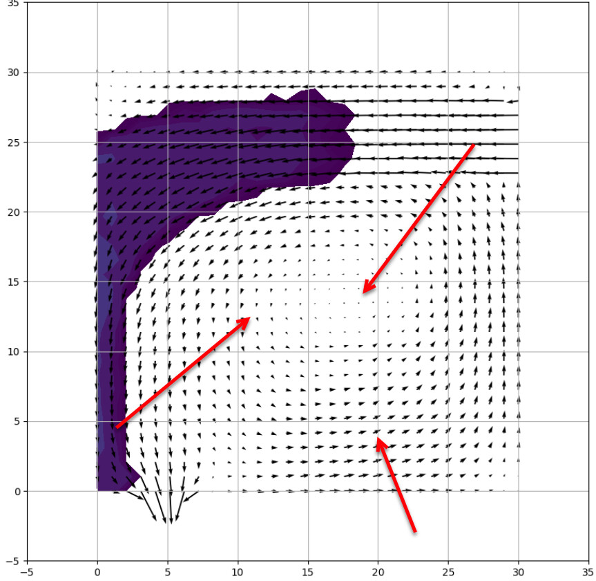
This simulation(the attached image) was generated using Python. I set the position at (1.5, 2.5) as the center and distributed particles (contaminants) within the radius of the cylinder in the model. The diffusion of particles is updated at each timestep, and I set the total number of steps, which equals the total simulation duration (steps * timestep(sec)). Additionally, I introduced a turbulence value of 0.1 at each timestep. I believe this approach may be more reasonable.
The difference is that I conducted a 2D simulation instead of 3D, and initially did not consider viscosity.
When would one need to use momentum sources?
Thanks for your help, and I will try changing the outlet to a pressure boundary condition.
Regards,
Chao Nien
Here are the results of my simulation run.
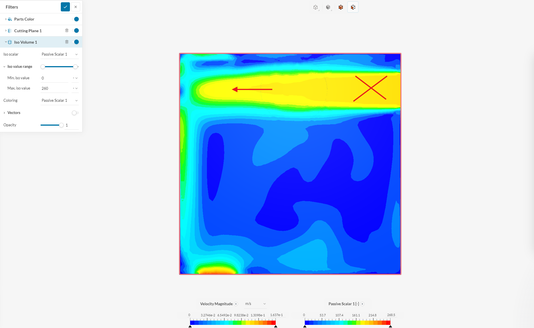
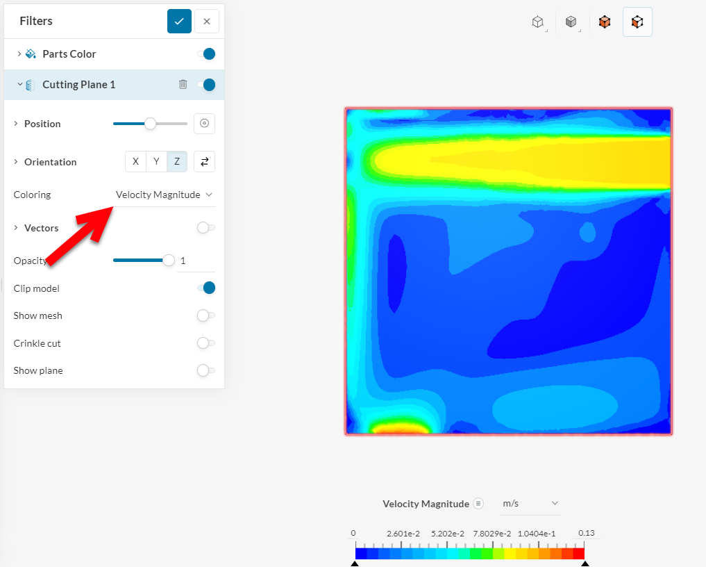
In this iteration, I removed the momentum source and adjusted the outlet to a pressure boundary condition. However, what I would like to ask is, as shown in the screenshot, shouldn’t the yellow area not appear at the inlet, since the contaminated area is set within the cylindrical bodies?
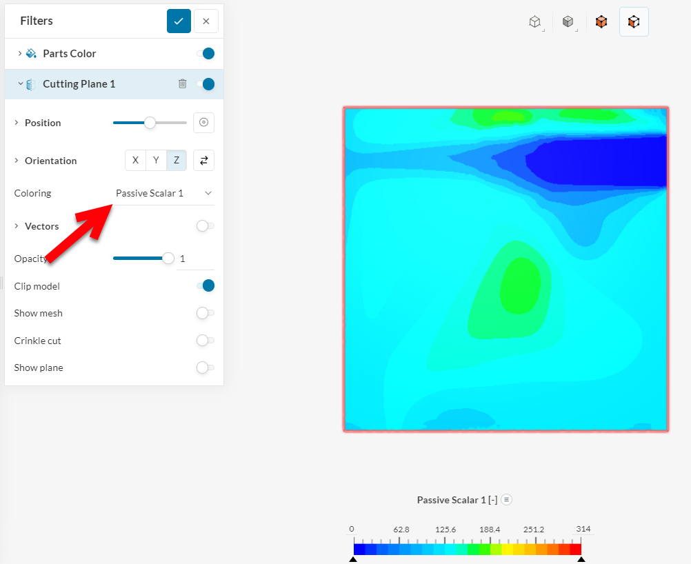
Hi @eaglechen, regarding your last question, could be because the definition of the coloring for the cutting plane is “Velocity” and not “Passive Scalar”?
When I take at a cutting plane for velocity, it looks like yours:
The transient solution would be one that varries in time. In your case, you have a Steady-State solution so that you should be expecting the result for the stabilized flow. To change that, you’d just need to change this option:
I think the image represents a transient solution because the passive scalar wasn’t diffused to other parts of the room, as should be expected in the stabilized flow.
Yes, that would mean it’s a transient analysis, since the values should be changing for each timestep!
That should be alright
A momentum source is used when there is, for example, a zone within the domain in which the fluid accelerates (such as a jet fan, present in the tutorial you initially pointed to).