Kindly refer to this link for the CAD model: Gas water heater venting malfunction - CO hazard by Ricardopg | SimScale
Overview
Gas water heaters are commonly used in residential buildings as an alternative to heating elements in electric showers. When poorly maintained, vented or installed, they can pose a threat to humans.
Carbon monoxide is a poisonous, odorless, colorless and tasteless gas. It results from the fuel burning in the water heater. Under normal circumstances, CO is vented out of the building through a chimney, preventing it from spreading in the interior. If this process is stopped, the CO becomes a potential hazard.
In this tutorial, making use of passive scalar transport, we are going to carry out a steady state CFD analysis of a gas water heater with a venting malfunction.
Step-by-step
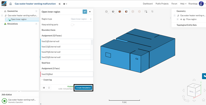
1) Create an open inner region
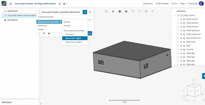
There’s a total of 3 openings in the model. First, the boundary faces have to be selected. Select the edges of all 3 windows as shown below:
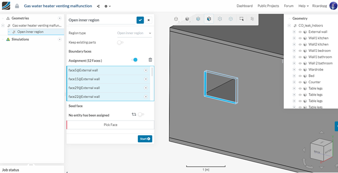
For the seed face, pick any face in the interior of the house.
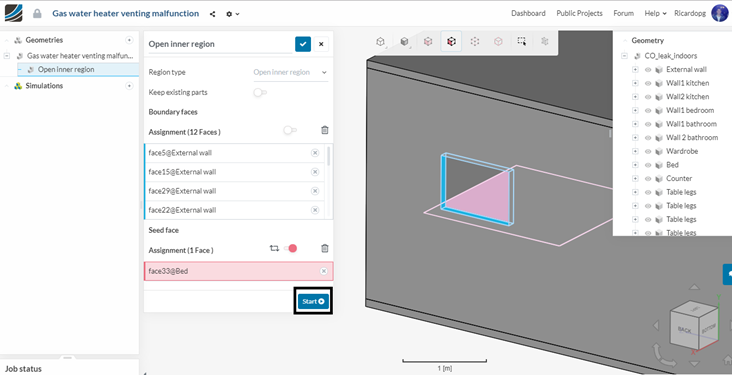
After setting up both the boundary faces and the seed face, give a click on Start to create the flow domain.
2) Create a simulation
When the operation finishes, click on create simulation and select Incompressible:
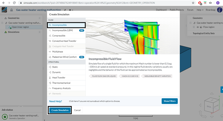
After clicking on Create Simulation, a simulation tree is open in the left panel. This tree shows sections where you will be able to configure the simulation. Sections ticked in green indicate that they have been filled up completely and no extra information is required. Sections marked as red indicate that they are not fully set.

3) Create a mesh
When creating a mesh, we must keep in mind that an accurate representation of our geometry is vital. Also, we have to make sure that the mesh is fine enough to capture the phenomena of interest that is going on within the flow. SimScale disposes of automatic and manual meshing tools. For this simulation, we are going to use a hex-dominant, automatic mesh.
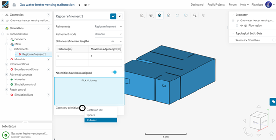
But first, we will set up a region refinement to better capture the source volume of carbon monoxide.
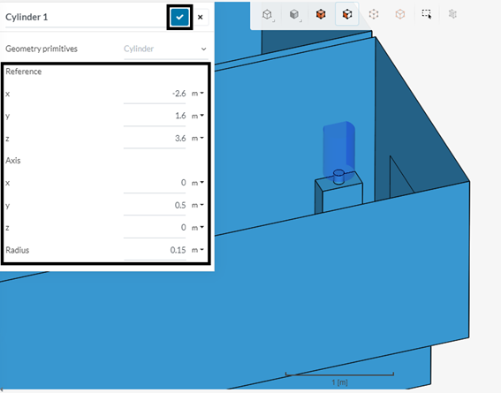
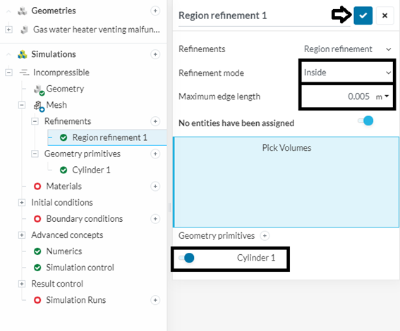
To do that, click on the “+” sign next to refinements and select region refinement. Click on the “+” sign next to geometry primitives and select a cylinder:
Give the following coordinates to the cylinder and click on the blue mark to save.
Now back to the region refinement tab, set up the refinement as shown below and then save it by clicking on the blue mark:
Now create an inflate boundary layer refinement by clicking again on the “+” sign next to Refinements and selecting Inflate boundary layer. We want to select all walls to be refined. Instead of selecting walls one by one, there’s an easier way to do this task.
Select the 3 outlets as shown in the figure below, then right click and invert the visible assignment:
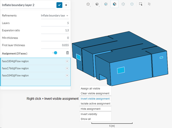
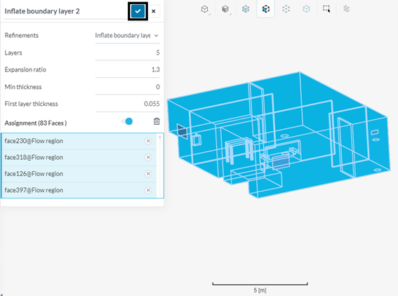
Then all walls are going to be automatically selected. Give a click on the blue mark to save:
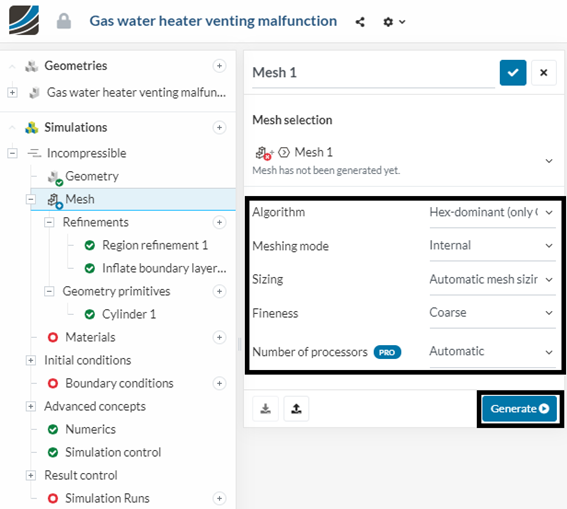
Now, in the left panel, click on Mesh. We are going to use a Hex-dominant mesh with automatic mesh sizing. After configuring your mesh, click on generate:
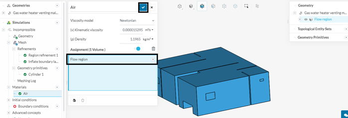
4) Assigning material
In the simulation tree, click on Materials and select air. Hit apply to confirm. Air is automatically assigned to the flow region. Once again, click on the blue mark to confirm:
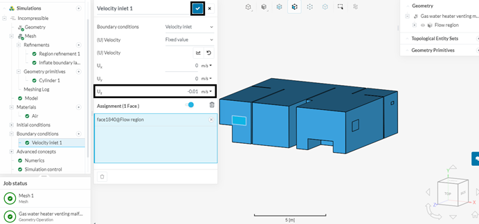
5) Setting up boundary conditions
Moving on to Boundary conditions in the simulation tree, click on the “+” sign and select velocity inlet. We are going to pick the kitchen window, which is located next to the water heater. We’re going to assume a very small, almost stale breeze. Notice the negative sign in Uz, as air is supposed to go into the flow domain:
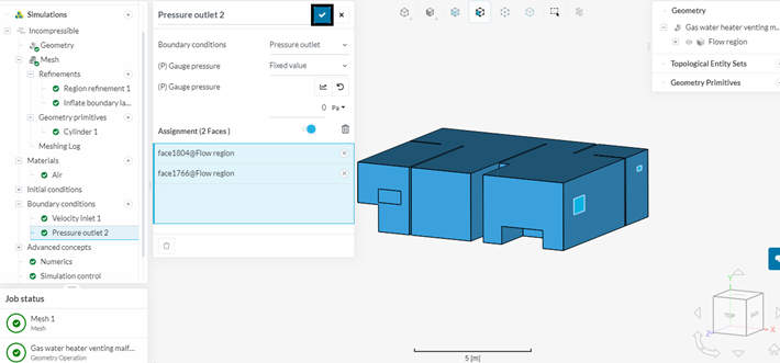
Let’s now set a pressure outlet boundary condition, by clicking on “+” and selecting pressure outlet. Select the other 2 windows, with 0 Pa fixed pressure and save:
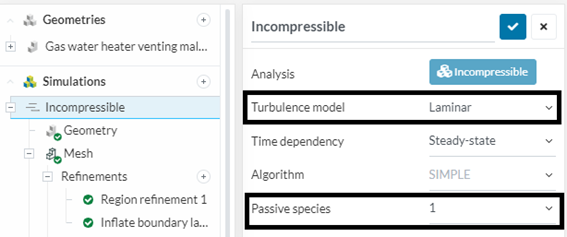
6) Passive scalar configuration
Now we can proceed to configuring our passive scalar source. First, in the simulation tree, click in Incompressible and select 1 passive scalar. Also change the turbulence model to Laminar as we’re going to work with very small velocities (and, therefore, low Re number):
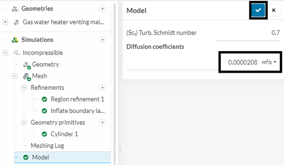
Click in a new tab that opened in the simulation tree named Model. Here you can set up diffusion coefficients. The diffusion coefficient of CO in air is 0.0000208 m²/s at 293.15 K:
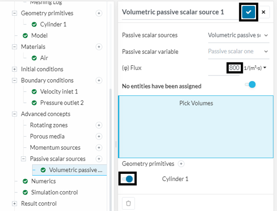
We will now setup the passive scalar source. In the simulation tree, click on Advanced concepts to enlarge, then click on Passive scalar sources and select Volumetric passive scalar source:
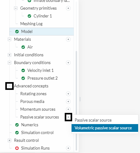
With this type of passive scalar source, we are going to generate certain quantity of passive scalar (it can be Kg, mL, molecules, L, ton etc.) per cubic meter of source volume per second . The chosen unit doesn’t change the result as long as you keep your units consistent throughout the setup and the post processing. For more information on passive scalar sources, please check the passive scalar transport documentations here and here for the sources documentation.
For this simulation, we are going to choose the unit that is the most convenient for the post processing: parts of CO per million parts of air (ppm).
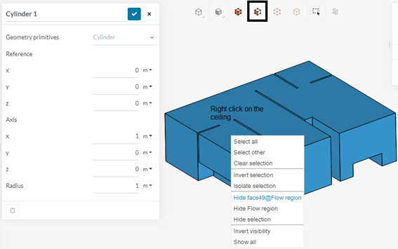
Click on the “+” sign next to geometry primitives. Select a cylinder. First let’s hide the ceiling of our house so we can properly place our passive scalar source.
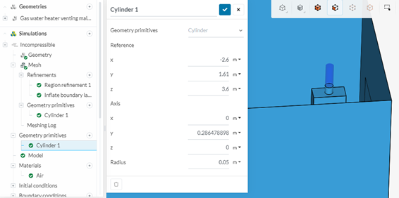
This volume corresponds to 2.25 liters and the cylinder was placed on top of the exhaust, where the venting duct was disconnected.
The permissible levels of CO in the flue vary from place to place. In the USA, for example, older water heaters can generate up to around 400 ppm of CO. In Brazil, up to 1000 ppm is considered acceptable. For this simulation, we’re going to assume 800 ppm of CO in the exhaust gas.
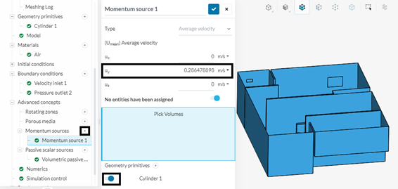
To replicate the effect of the exhaust gas leaving the water heater, we are going to set a momentum source to the passive scalar source.
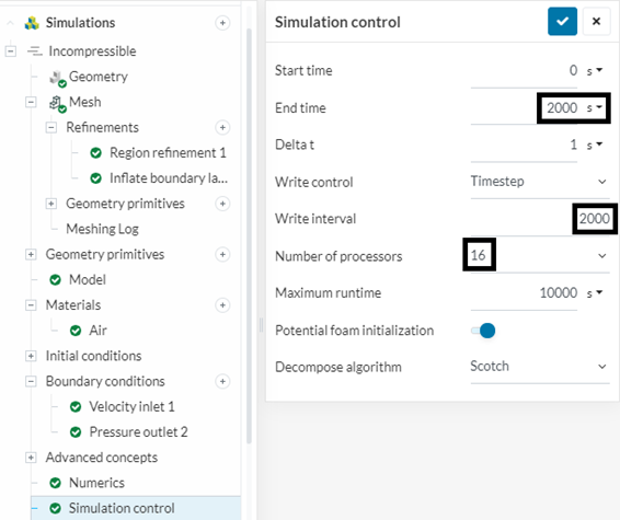
7) Simulation control and result control
Select a 16 processors machine to run this problem, as the mesh has around 2.4M cells.
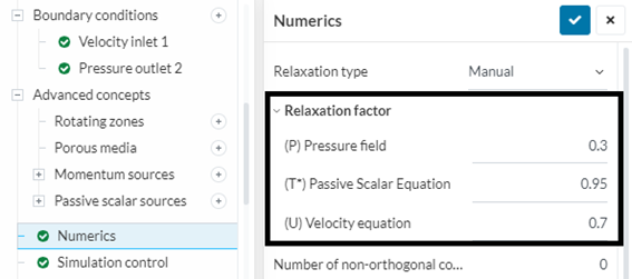
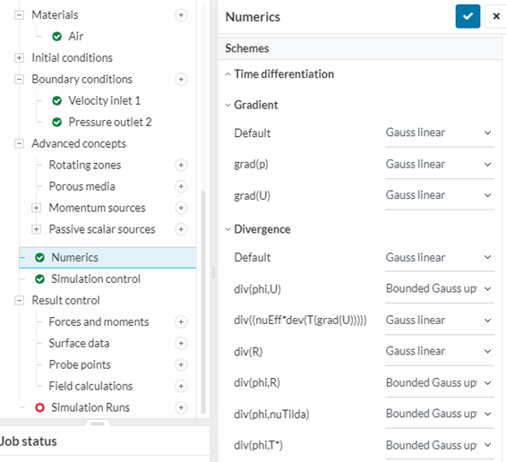
Click on the Numerics tab in the simulation tree. Change the relaxation factors to the following:
Now, still in the numerics tab, scroll down until the schemes section. For the gradient schemes, select Gauss Linear to all entries. Select the divergence schemes as shown below:
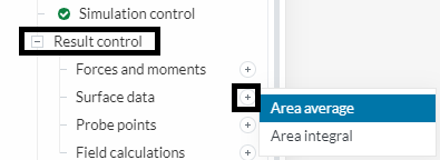
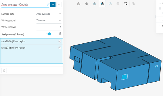
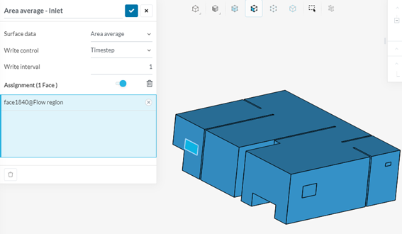
In order to help us assess convergence, we will set area average controls for both outlets and the inlet:
Now we are ready to run the simulation. Click on the “+” sign next to Simulation Runs. There will be a warning message saying that a relaxation factor greater than 0.7 for the passive scalar term can cause instabilities. This won’t happen in this specific simulation. So, we will proceed by clicking on Ok and Start.
8) Results
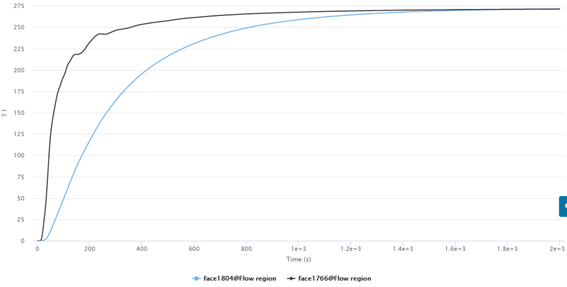
We can use the result control that we set previously to help in assessing convergence. Go to the following directory in the simulation tree:
We can see that the passive scalar levels (T1) at the outlet are converging to a value:
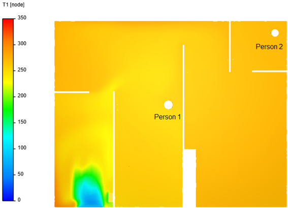
Exposure limits given by the American Conference of Governmental Industrial Hygienists (ACGIH) are often taken as a benchmark when it comes to chemical substances. Carbon monoxide, according to ACGIH has a time-weighted-average (TWA) exposure limit of 25 ppm. This is a level that most workers can be exposed for 8 hours straight without having adverse health effects.
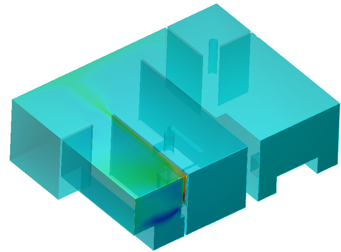
For the present case, the exposure levels reach upwards of 250 ppm in the whole building. Short term exposure to these concentrations can cause cardiac effects on susceptible populations.
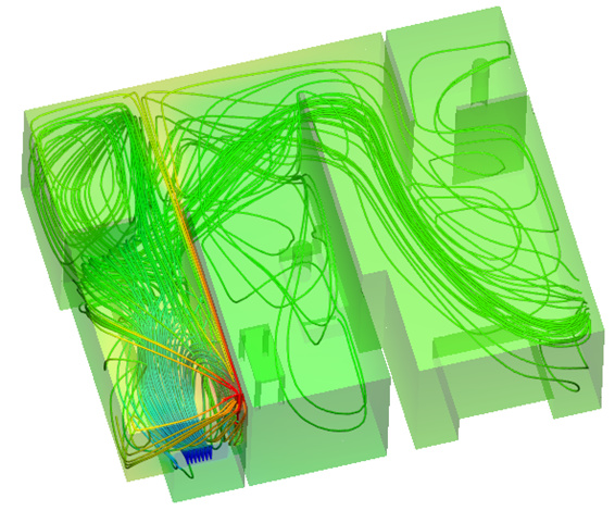
It’s worth noting that if the inlet flow rate would have been lower (eg. if the kitchen window were shut), the ppm levels inside the building would grow exponentially, reaching deadly levels in a short period of time.