Recording

Homework Submission
For your homework, your task is to investigate the behavior of drag and lift, and look at velocity and pressure distribution across the wing for different angles of attack (which will be simulated without changing the geometry). We will work with an angle of 3 degrees, and 20 degrees for a plane travelling at 20 m/s.
The step-by-step tutorial below contains all of the steps for setting up the simulation in SimScale and visualizing the results.
To submit your homework assignment, please generate a public link of your project (Sharing a Project)
Homework Deadline: December 10th, 11:59 pm CEST
Click Here to Submit your Homework
Outline
PART 1:
-
Introduction
-
Project Import
-
Mesh Generation
a. Geometry Primitives
b. Mesh Refinements
c. Start Operation
d. Mesh Quality -
Simulation Setup (AOA = 3)
a. Simulation Setup
b. Domain
c. Material
d. Initial Conditions
e. Boundary Conditions
f. Numerics
g. Simulation Control
h. Result Control (Lift & Drag)
i. Simulation Runs -
Recommendations About Comments
PART 2:
-
Simulation Setup for Different AOA
a. Duplicating Simulation
b. Boundary Conditions
c. Lift & Drag -
Post-Processing
a. Filters/Visualization
b. Additional Features -
Recommendations About Comments
Introduction
In this tutorial, you will be doing a full fledged flow simulation of the aerodynamics of a model airplane. The focus of this simulation is to investigate the performance of the airplane - in particular the wing - by looking at drag and lift forces at different angles of attack.
For your homework, your task is to investigate the behavior of drag and lift for different angles of attack (which will be simulated without changing the geometry) and determine the best setup. We will work with an angle of 3 degrees and 20 degrees for a plane travelling at 20 m/s.
Let’s take a look at the physics of the plane before we start to set up our simulations.

This is how our plane will look in real life, but as standard practice for simulations we can make some simplifications.

As a first simplification we can exploit the symmetry of the plane. Simulating only half of the plane reduces the computational effort by defining the inner surrounding wall (yellow/brown) as a symmetry plane.
The body of the plane is a physical wall (grey), which means that it involves friction and should be defined as so-called no-slip walls.
The outer (not visible here), upper, and lower surrounding walls (dark blue) are necessary to limit the size of the domain we want to simulate since we are not able to simulate an infinitely large domain. In reality, these walls do not exist and should not interact with the flow. A good approximation here is to assume this wall as frictionless or so-called slip walls.
The bounding face on the right-hand side (red) will be defined as an inlet with a constant flow velocity profile.
The bounding face on the left-hand side (green) will be defined as an outlet with a constant pressure.
These four bounding walls define the size of the fluid domain, and in general you have to reach a compromise: you want these walls as far as possible so that you can observe all the fluid behavior (also, if they are too close to your geometry you might get strange results), but you also want to limit your fluid domain to save computational power.
You will simulate three different set-ups with the geometry provided in the project.
First we will go through the meshing process, as the same mesh will be used for all simulations. Then we will talk about the standard setup for the simulation, and then we will go into the setup to change the angle of attack. This will be done by changing the angle of incidence of the air, and we will dig deeper into this later on.
General notes:
- Most of the descriptions will be below the images.
- For many attributes, SimScale sets some default values that don’t need to be changed unless specified. Please double check your procedure with the screenshots and text
Project Import
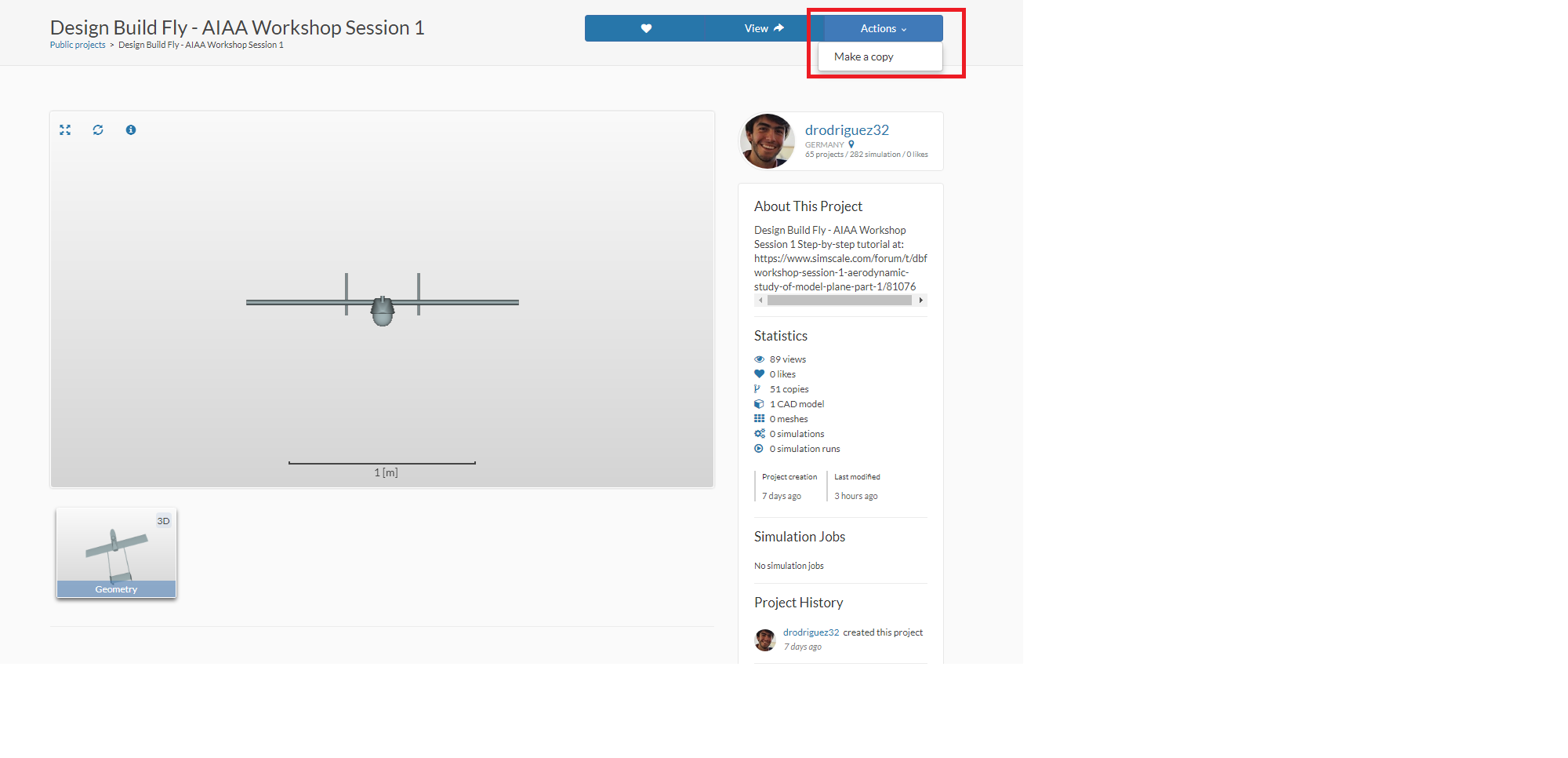
To start this exercise, please import the project into your workspace by clicking on the link below:
If the project appears to be private, please make a copy of it to work on it.
Mesh Generation
For this tutorial we will work with an airplane with a standard angle of attack of 3 degrees and an H configuration for the tail.
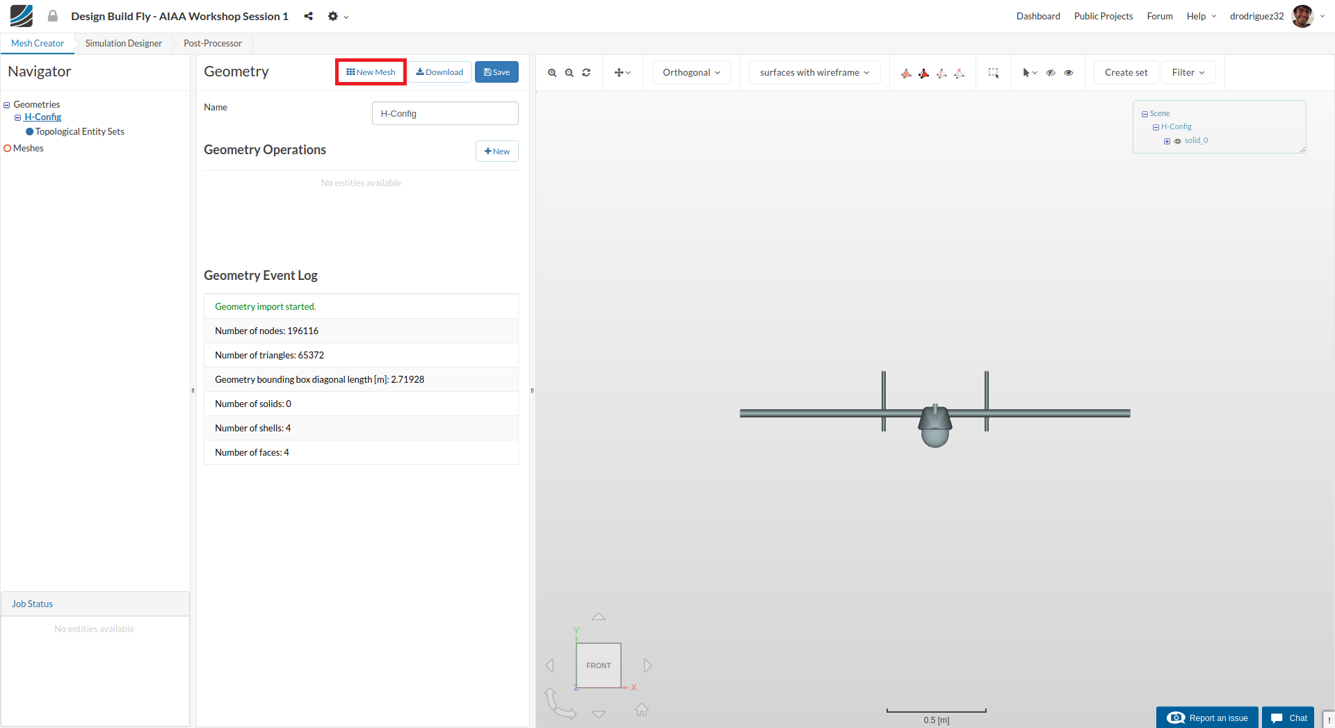
Start by clicking on the H-Config model under Geometries in the navigator. Then click on New Mesh to start creating a new mesh on this geometry (this doesn’t start the mesh operation, you still have to go through all the settings).
The new mesh operation will be generated automatically. Next change:
-
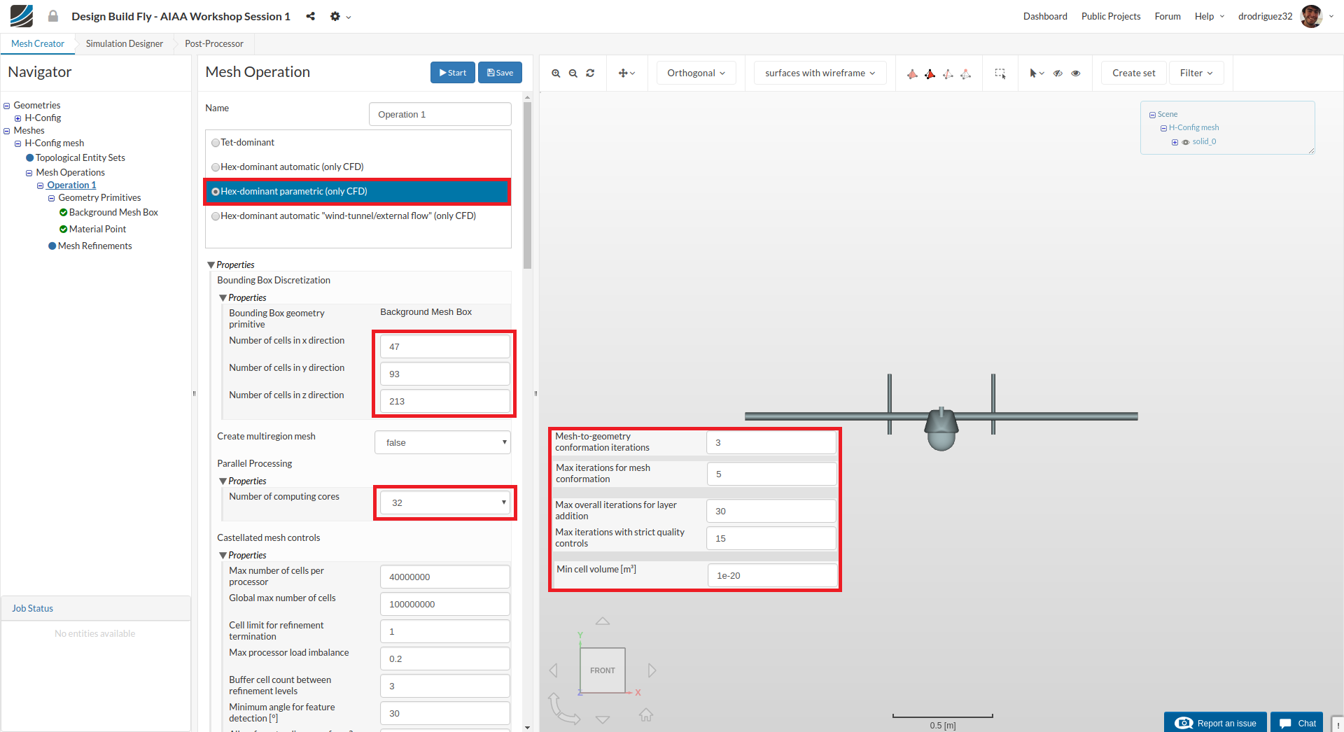
Set the Type to Hex-dominant parametric (only CFD).
-
Configure the Bounding Box geometry primitive to the following:
Number of cells in x direction to 47
Number of cells in y direction to 93
Number of cells in z direction to 213Here you are refining what is known as the level 0 refinement, or the coarsest mesh that will exist in your model. The bounding box refers to a setting you will modify in a few steps and something we already talked about in the introduction: the fluid domain. So with this you are specifying into how many control volumes you would like to split your model. SimScale generally generates a good number by default, but you are free to change it (like we do here). You have to be careful because you don’t want a mesh that’s too coarse to be solved properly but you also don’t want a mesh that’s too fine for areas where the flow is very simple.
-
Set the Number of parallel computing cores to 32
-
Scroll down to change other values to optimize the meshing parameters
-
Mesh-to-geometry conformation iterations to 3
-
Max iterations for mesh conformation to 5
-
Max overall iterations for layer addition to 30
-
Max iterations with strict quality controls to 15.
-
Min cell volume [m³] to 1e-20
-
Click Save to register changes.
Geometry Primitives
Background Mesh Box
Next, under Geometry Primitives select Background Mesh Box.
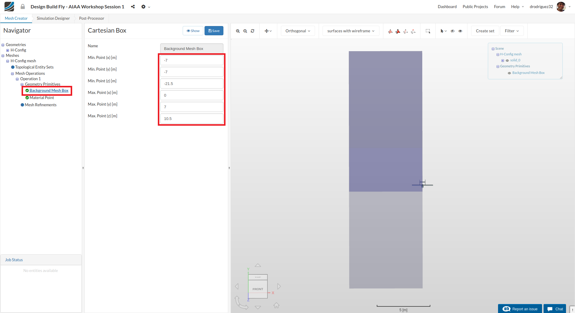
Change the setting accordingly:
- Min. Point (x) = -7
- Min. Point (y) = -7
- Min. Point (z) = -21.5
- Max. Point (x) = 0
- Max. Point (y) = 7
- Max. Point (z) = 10.5
Here you are defining the size of the fluid domain.
Click Save. If you don’t see the entire box click on the reset icon over the viewer to see the created mesh box.
Material Point
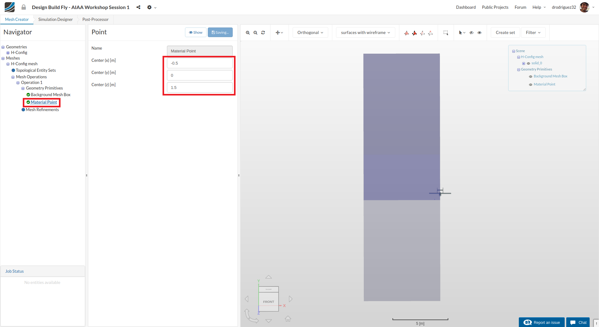
Next you will specify the material point. This will tell the platform where the mesh will be created, so make sure it is inside the Background Mesh Box but outside of any solid (if you leave it inside the plane the platform will think you want to do a simulation of the flow inside the plane). Input these values:
- center (x) = -0.5
- center (y) = 0
- center (z) = 1.5
Then click Save
Inner Box
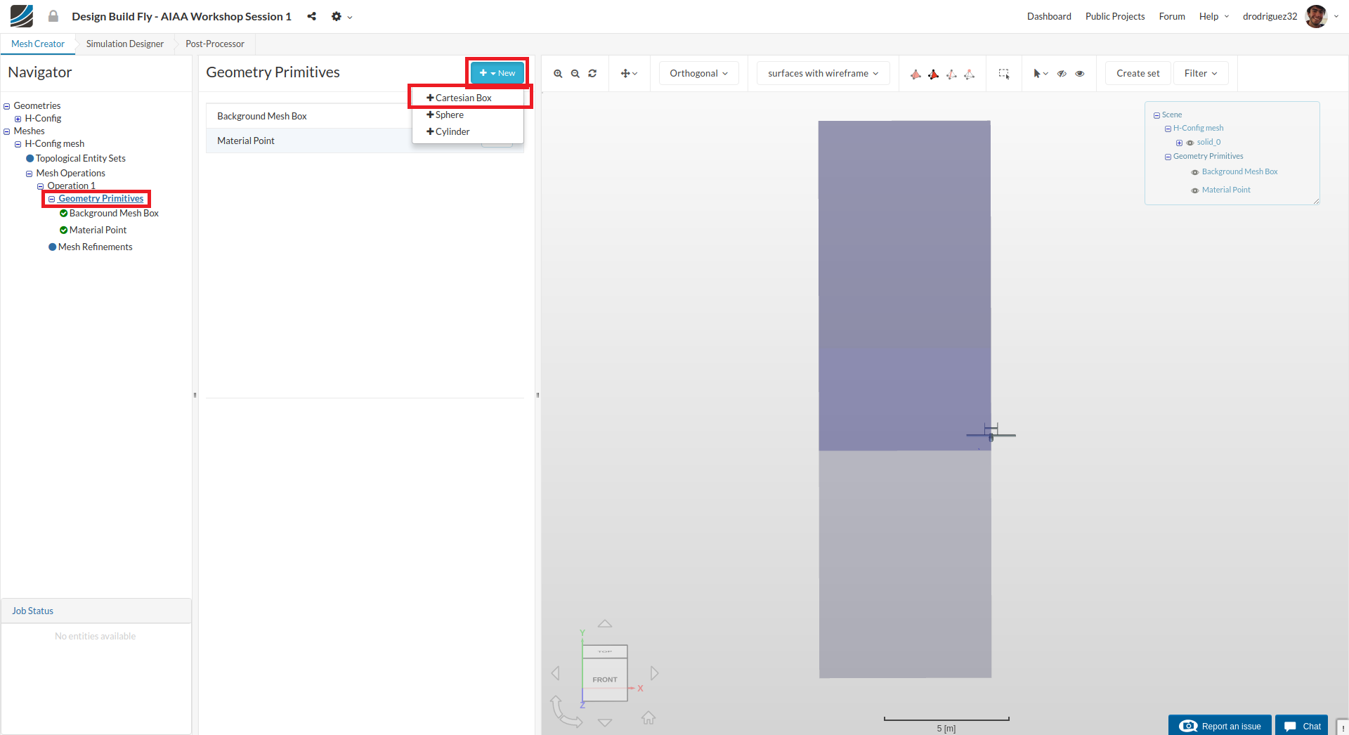
Next go back to Geometry Primitives and click on + New and then Cartesian Box to define a new Cartesian Box that will be used to define a mesh refinement region.
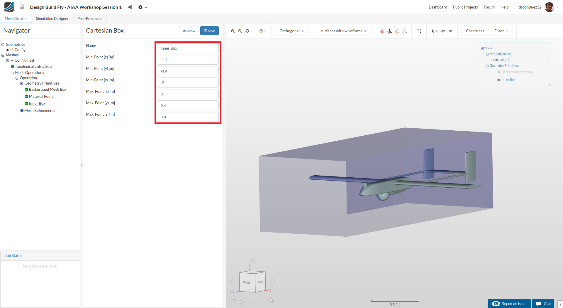
After creating a new Cartesian Box, you will be directed to the definition of this Cartesian Box. Change the dimensions of the box to the following:
- Min. Point (x) = -1.1
- Min. Point (y) = -0.4
- Min. Point (z) = -2
- Max. Point (x) = 0
- Max. Point (y) = 0.4
- Max. Point (z) = 0.8
Click Save to register your changes.
Fuselage Box
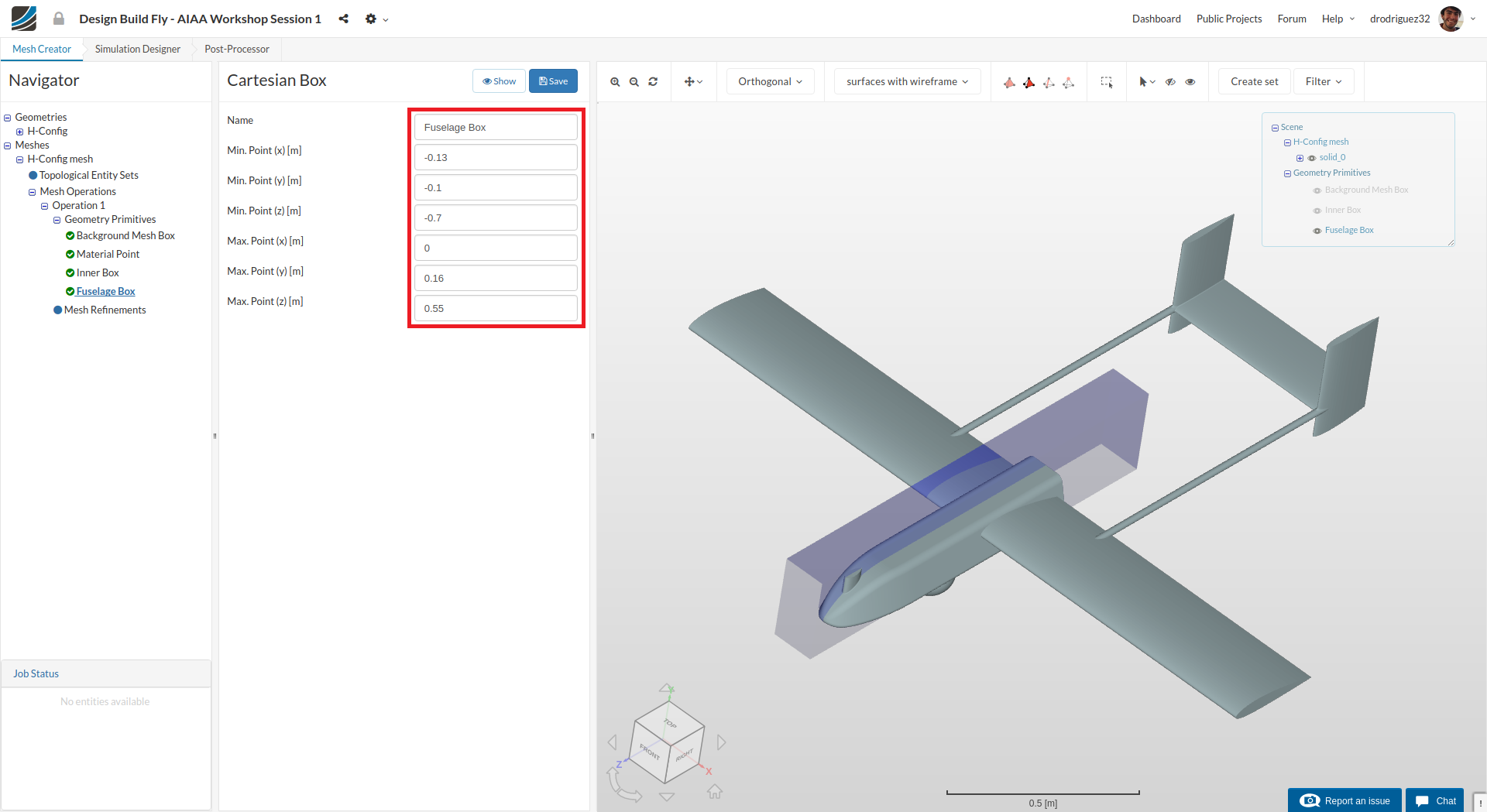
Follow the same procedure to define another Cartesian Box for further refinement definitions. Rename it to Fuselage Box. This time change the values to the following:
- Min. Point (x) = -0.13
- Min. Point (y) = -0.1
- Min. Point (z) = -0.7
- Max. Point (x) = 0
- Max. Point (y) = 0.16
- Max. Point (z) = 0.55
Click Save to register your changes
Wings Wake
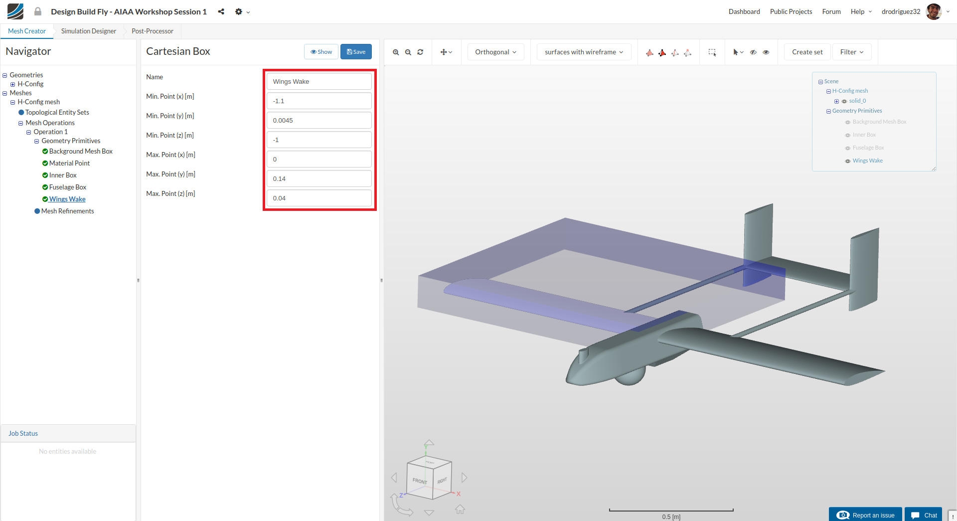
Define another Cartesian Box for further refinement definitions. Rename it to Wings Wake. Change the values to the following:
- Min. Point (x) = -1.1
- Min. Point (y) = 0.0045
- Min. Point (z) = -1
- Max. Point (x) = 0
- Max. Point (y) = 0.14
- Max. Point (z) = 0.04
Click Save to register your changes
Tail Wake
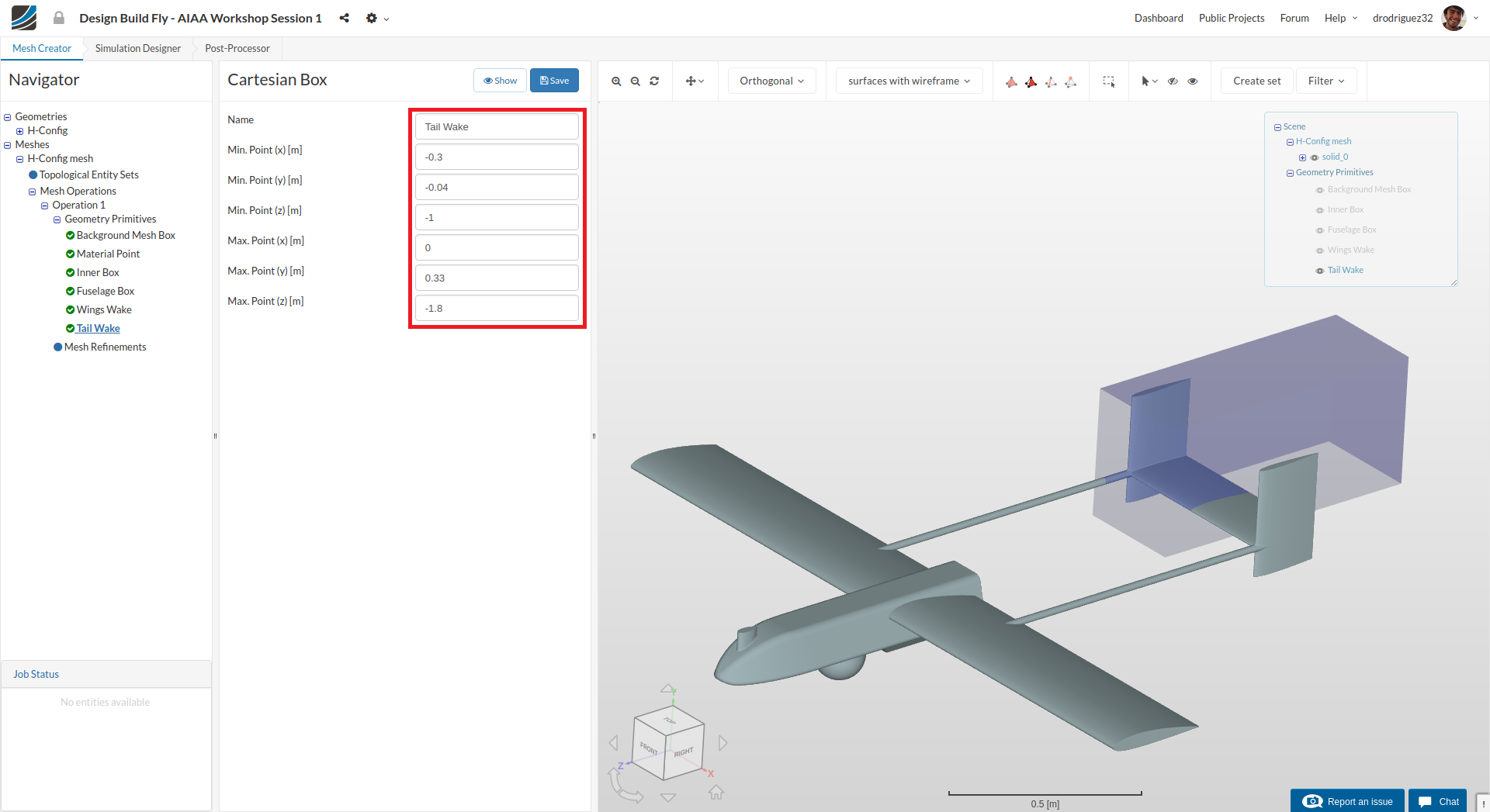
Define another Cartesian Box for further refinement definitions. Rename it to Wings Wake. Change the values to the following:
- Min. Point (x) = -0.3
- Min. Point (y) = -0.04
- Min. Point (z) = -1
- Max. Point (x) = 0
- Max. Point (y) = 0.33
- Max. Point (z) = -1.8
Click Save to register your changes
With these Cartesian Boxes that we created we will define refinement regions where cells will be smaller and thus we will be able to observe more detail in the complex areas of the flow - a mesh that is too coarse will not allow you to observe small flow structures.
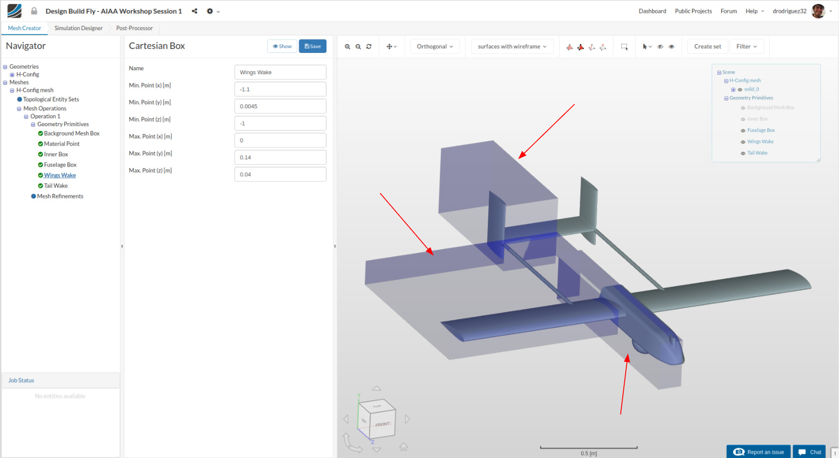
Notice that we have created these boxes around the plane geometry to better observe the behavior in close proximity to the airplane.
Mesh Refinements
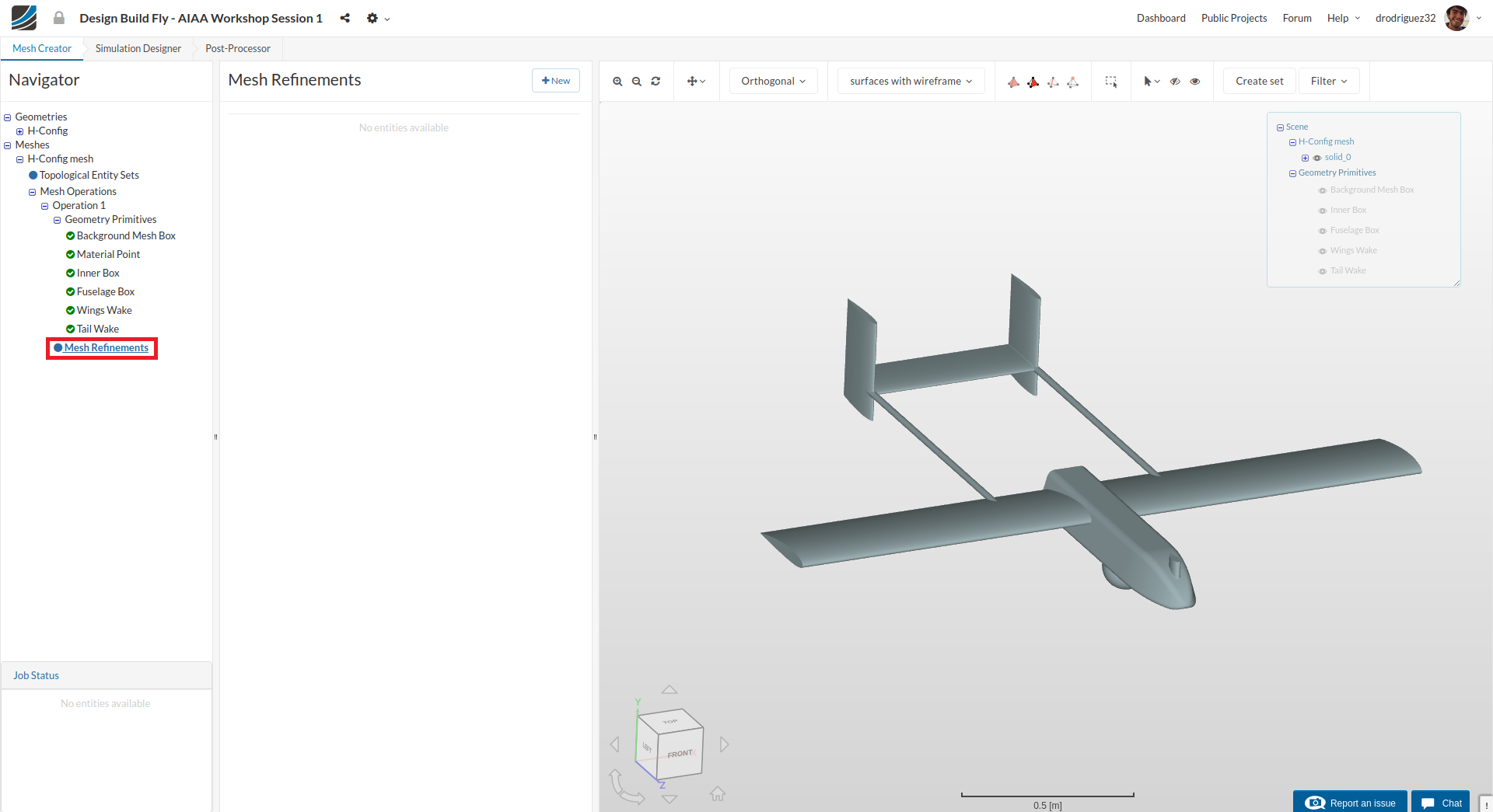
A good mesh requires well defined refinements. Now we will start creating the mesh refinements. For this proceed to Mesh Refinements and click +New
How does a mesh refinement work? It divides each cell to create more, smaller cells, and each level of refinement applies this to the cells generated in the past refinement level. This means that each cell that is refined will be divided into 4 smaller cells for each level. Example: at level zero you have 1 cell, at level one you have 4 cells, at level two you have 16 cells, at level three you have 64 cells, and at level four you will have 256 cells.
1. Plane Surface
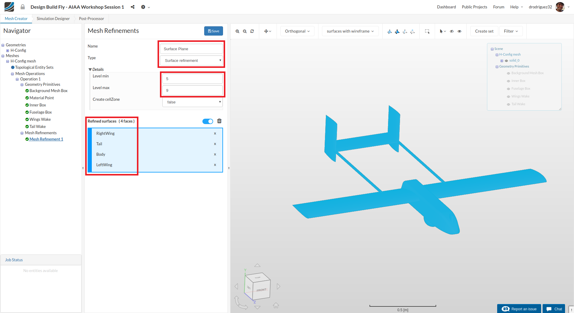
Rename it to Plane Surface (optional).
Change the Type to Surface refinement and then both Level min and Level max to 5 and 9 respectively.
Select all the parts of the plane (RightWing, Tail, Body, LeftWing).
With this refinement we are improving the mesh that sits directly on the surface of the geometry. We do this to capture more accurately more details of the geometry and to better observe how the flow interacts with the surface of the plane.
Click Save to register your changes.
2. Plane Region
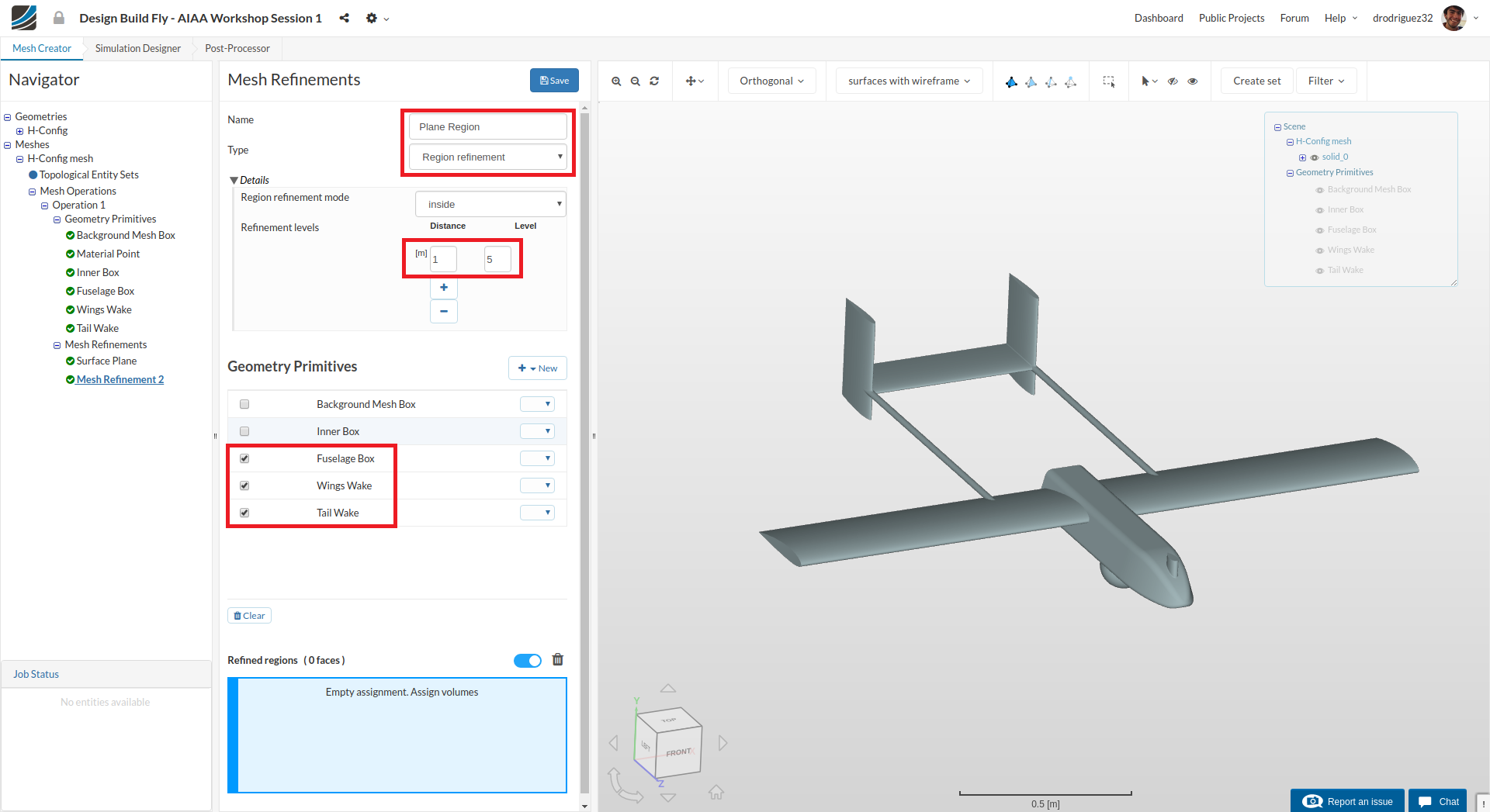
Now we will start refining the regions (Cartesian Boxes) that you created earlier.
Following the same procedure as before, create a new refinement and name it Plane Region (optional).
Change Type to Region refinement and then under Refinement levels change Level to 5
Select Fuselage Box, Wings Wake, and Tail Wake under Geometry Primitves and click Save to register the refinements for these specific Cartesian boxes.
This is the region closest to the plane, so flow structures will be more complex immediately around and after the geometry. So we want this area more refined.
3. Inner Box Region
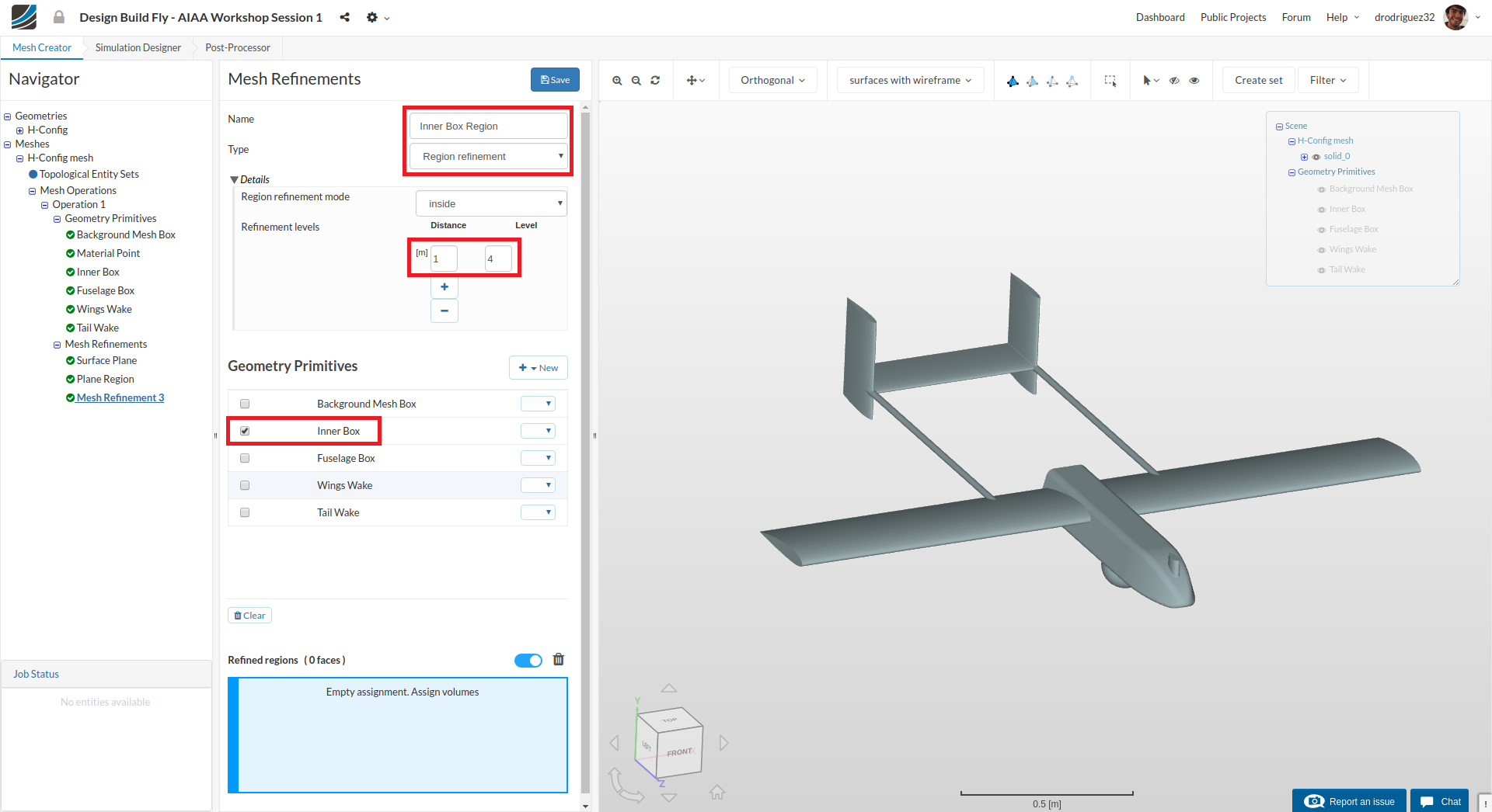
Create a new refinement for the final Cartesian Box. This time rename it to Inner Box Region (optional).
Change Type to Region refinement and then under Refinement levels change Level to 4
Select Inner Box under Geometry Primitves and click Save to register the refinements for this specific Cartesian box.
Further away from the plane we won’t have such complex flow, but because we are still considerably close and the flow is still affected we want this region slightly refined as well.
4. Layers
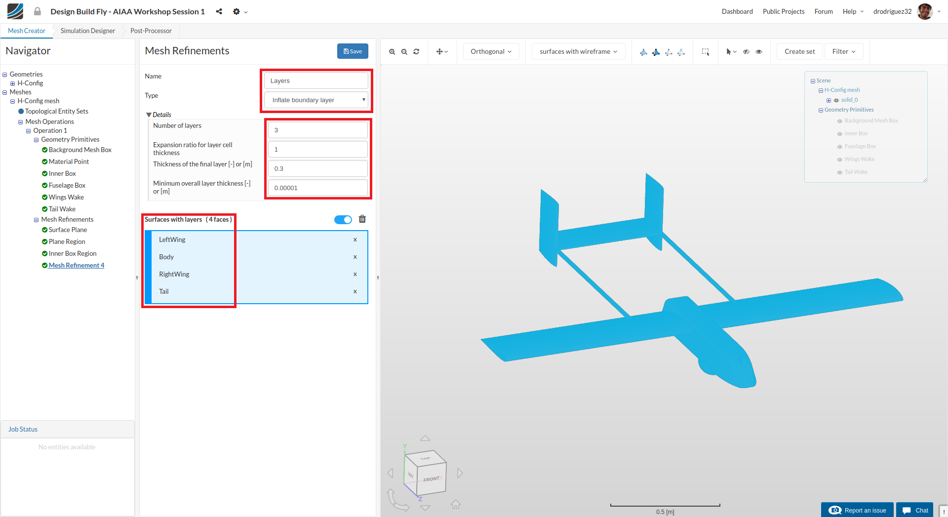
Next we will add layers over the surfaces on the whole plane. Layers will create small cells along every face of the geometry that copy and inflate the surfaces. and allow us to capture the results near the bodies (like the development of the boundary layer) more accurately.
Create a new refinement and rename it to Layers (optional).
Change Type to Inflate boundary layer and then change Number of layers, Expansion ratio for layer thickness and Minimum overall layer thickness [-] to 3, 1, and 0.00001 respectively.
The expansion ratio defines how fast the boundaries will grow - how much larger the next boundary cell will be compared to the past. And the minimum overall thickness defines a minimum limit to the size of the boundary layers - if the overall thickness is below this number, the algorithm will consider it not significant and no layers will be added.
Select all the parts of the plane. Under Surfaces with layers you should all four parts selected.
Click Save to register your changes.
Start Operation
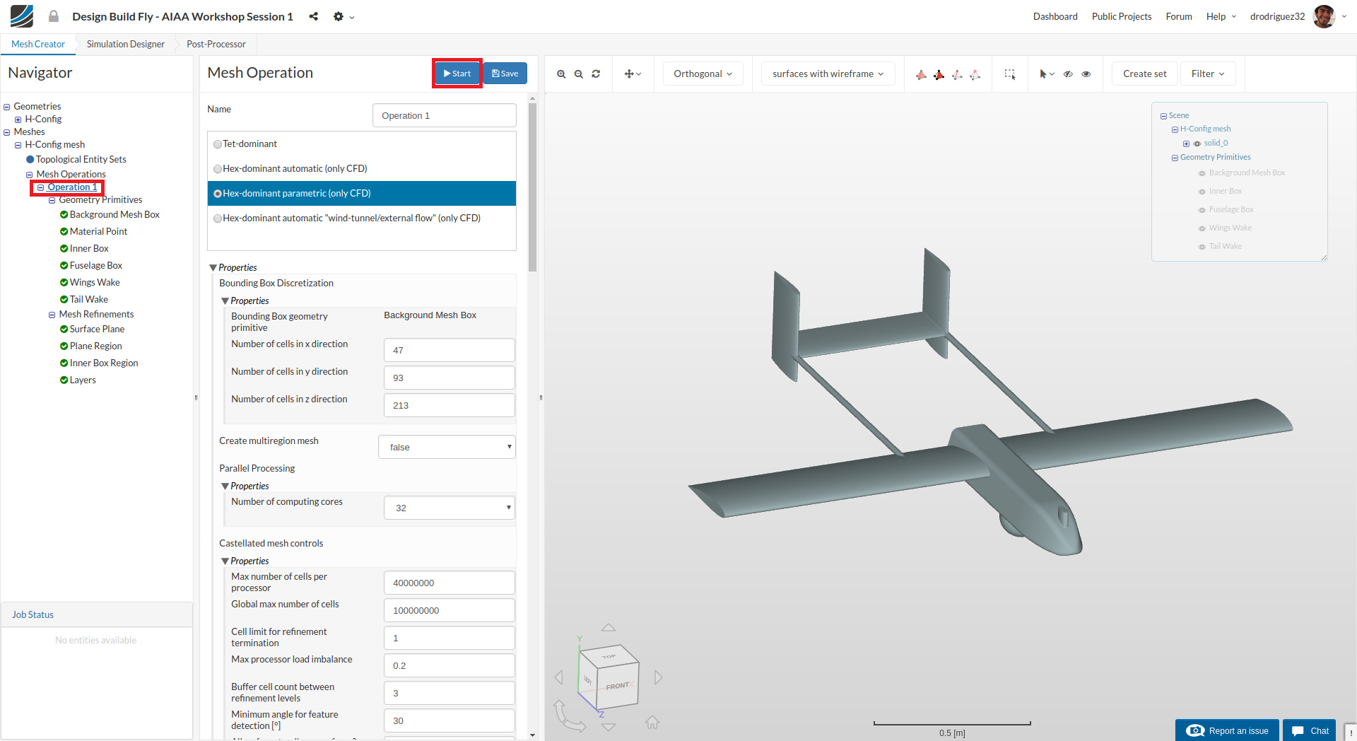
Once you have defined all of the mesh refinements, go back to the Operation 1 and click Start in order to submit the meshing job to the server. Due to the fineness of the mesh, the meshing could take around 71 minutes to finish. When the meshing is done you will see a green sign that says FINISHED when you click on your mesh.
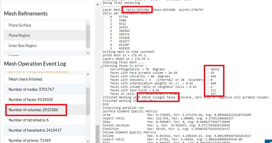
Mesh Quality
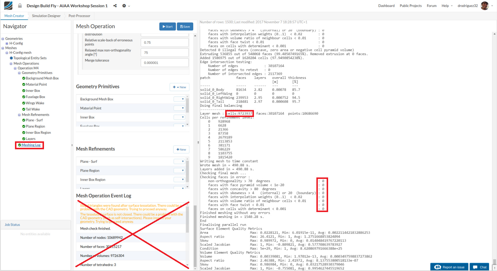
When your meshing process is done, don’t look at the Mesh Operation Event Log. If you want to check the quality of your mesh please click on Meshing Log in the Navigator and scroll to the bottom of the text log. There should be zero illegal faces (like in the picture), and your mesh should have around 9.7 million cells.
Simulation Setup (AOA = 3)
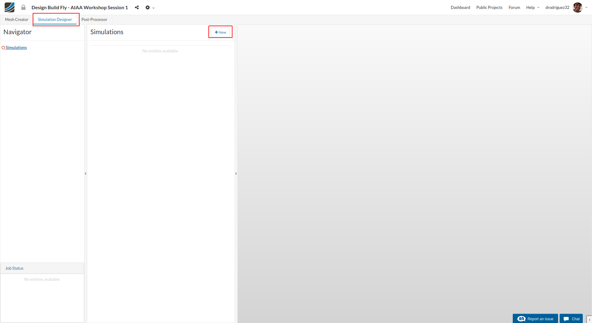
Once the meshing is finished, you can proceed to Simulation Designer to set up the simulation.
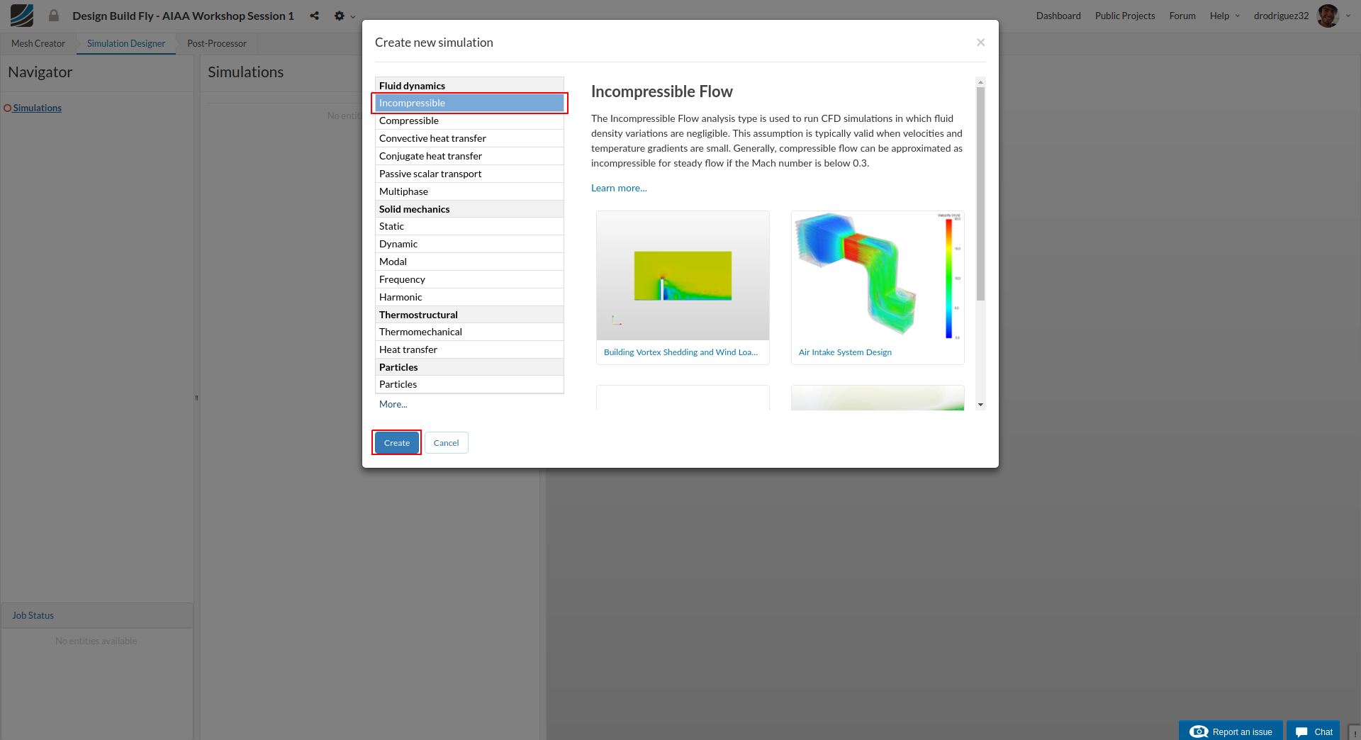
Once you are in Simulation Designer, click New Simulation in order to start setting up the simulation. A window will pop up where you have to select the Analysis Type. Under Fluid dynamics select Incompressible and click on Create.
Once you save the analysis type, you will see the expanded navigator tree. All the red entities shows that they must be set up in order to perform a successful simulation run.
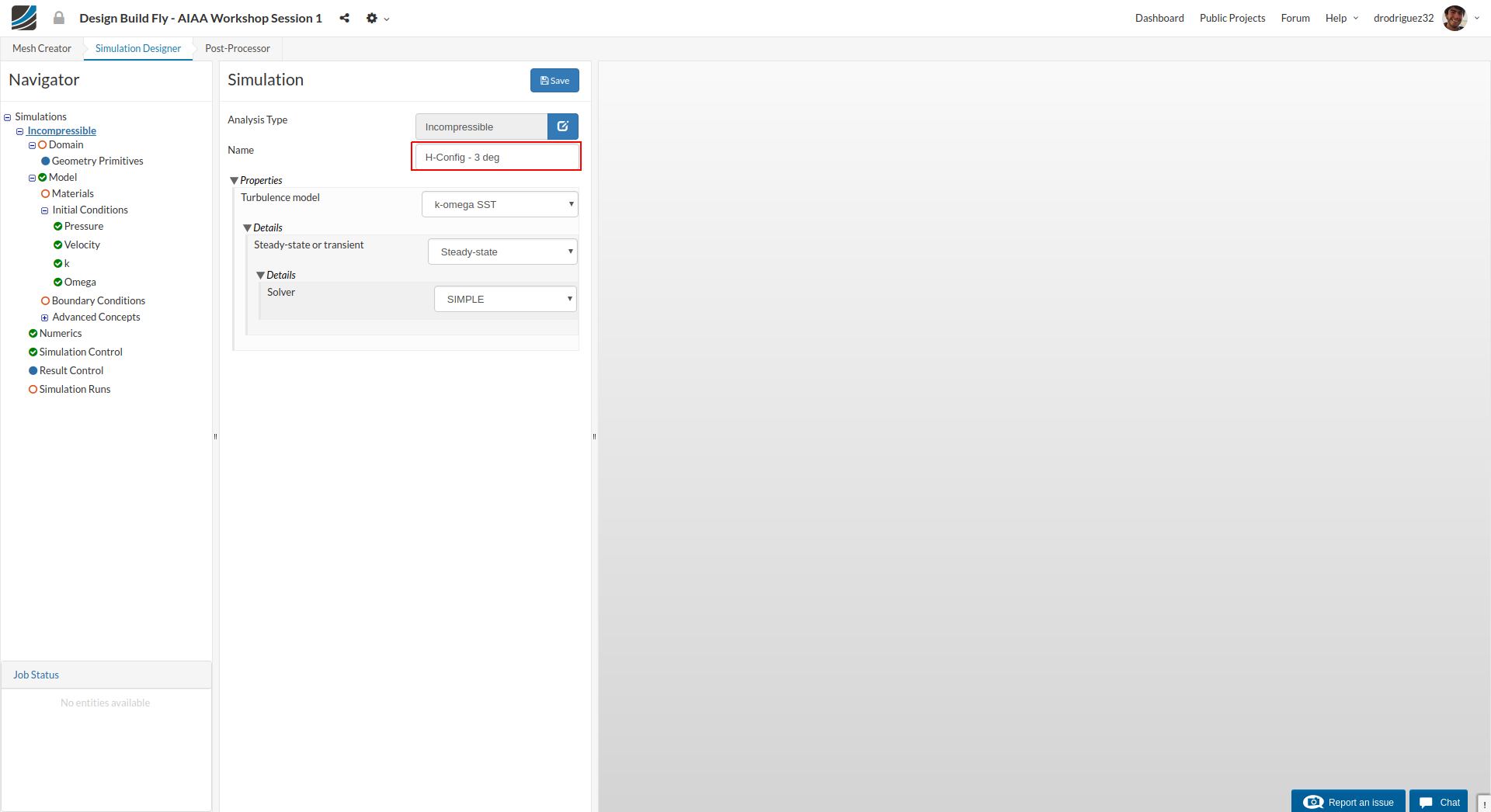
Rename your simulation to “H-Config - 3 deg” (optional) and click on Save
Domain
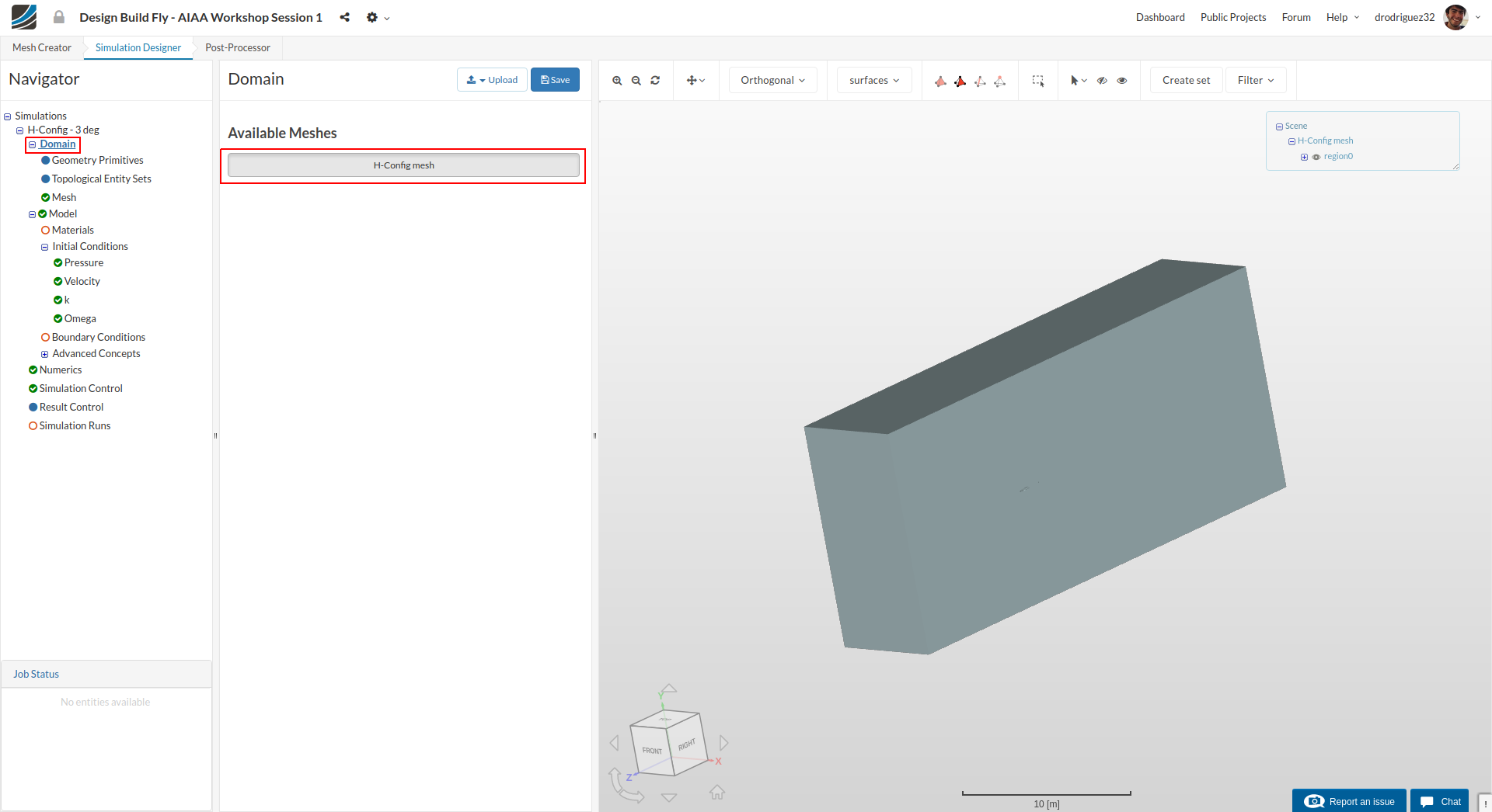
Next you have to select a domain on which this simulation will be performed. Proceed to Domain and select H-Config mesh and click Save.
After a while you will see the loaded mesh of the selected domain in the viewer. For the easier mesh handling, it is recommended to switch to the surfaces render mode in the top viewer bar.
Material

Next we have to define the fluid material. Go to Materials and click on +New to create a new material.
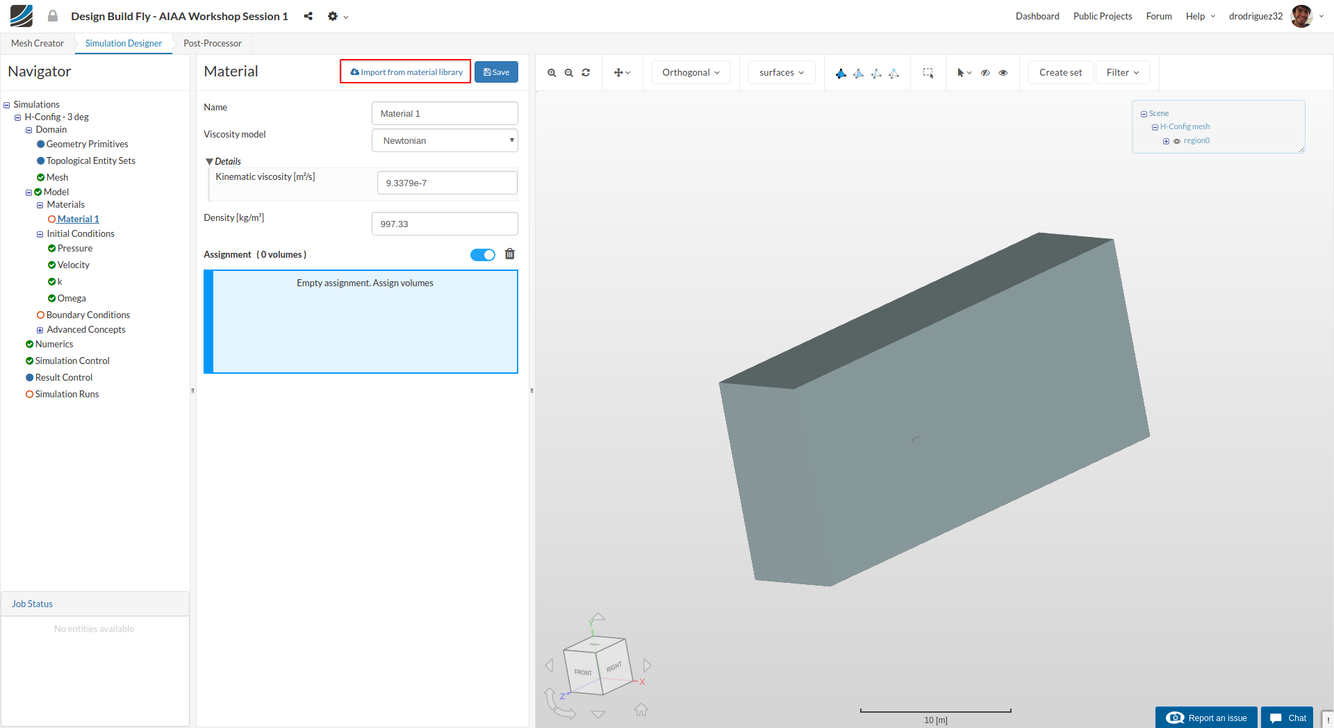
Click on Import from material library to import the desired material from the material database.
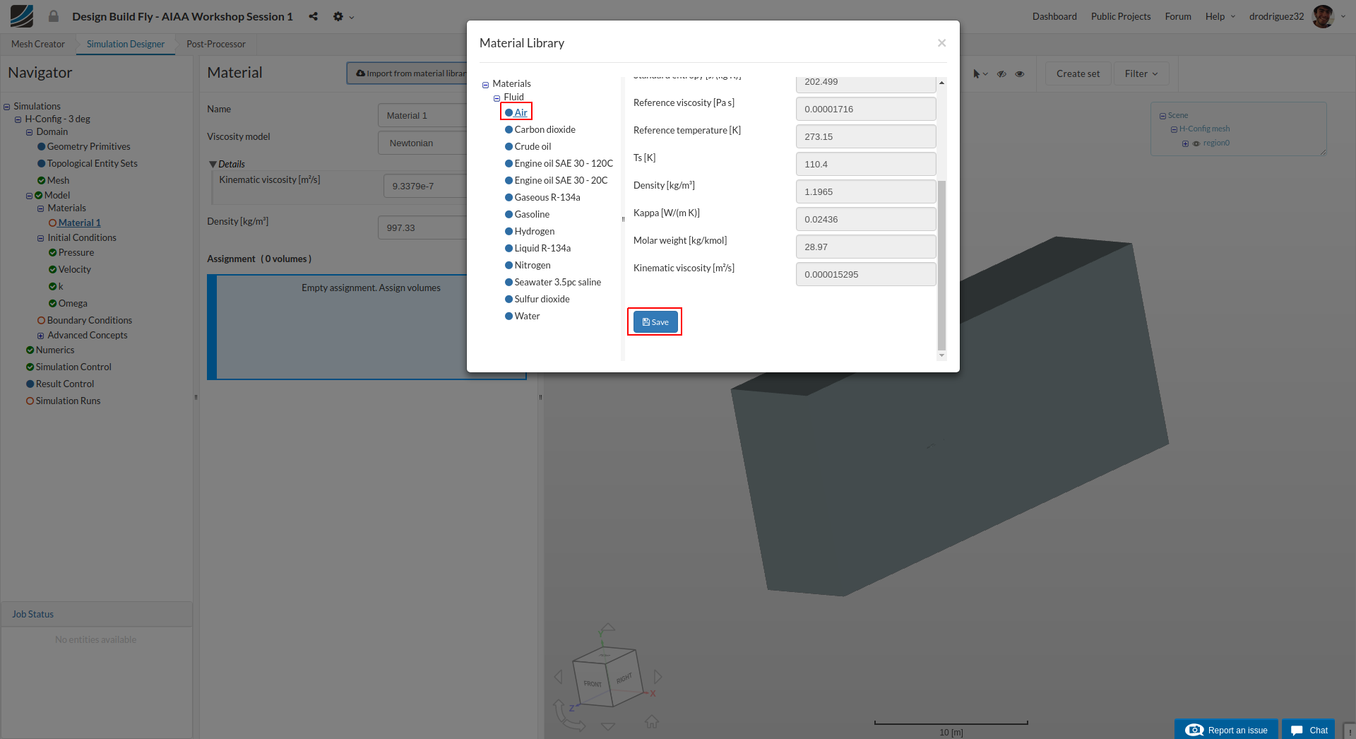
Select Air and click Save to import this material directly from the library.
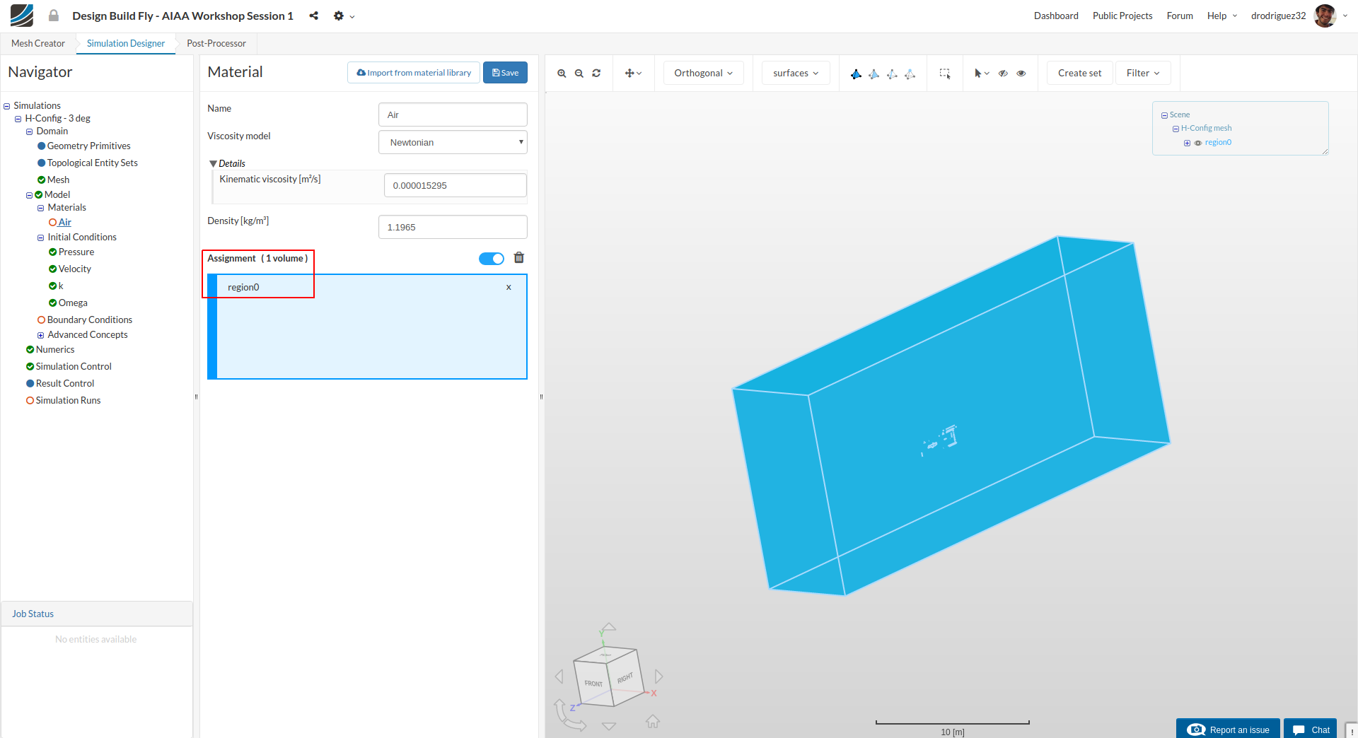
Click on your mesh in the viewer. You should see region0 under Assignment and then click Save in order to define the material for this region.
Initial Conditions
Pressure and velocity we will leave as the default set by SimScale.

Go to k and change the Turbulent kinetic energy value [m²/s²] value to 0.06 and click Save
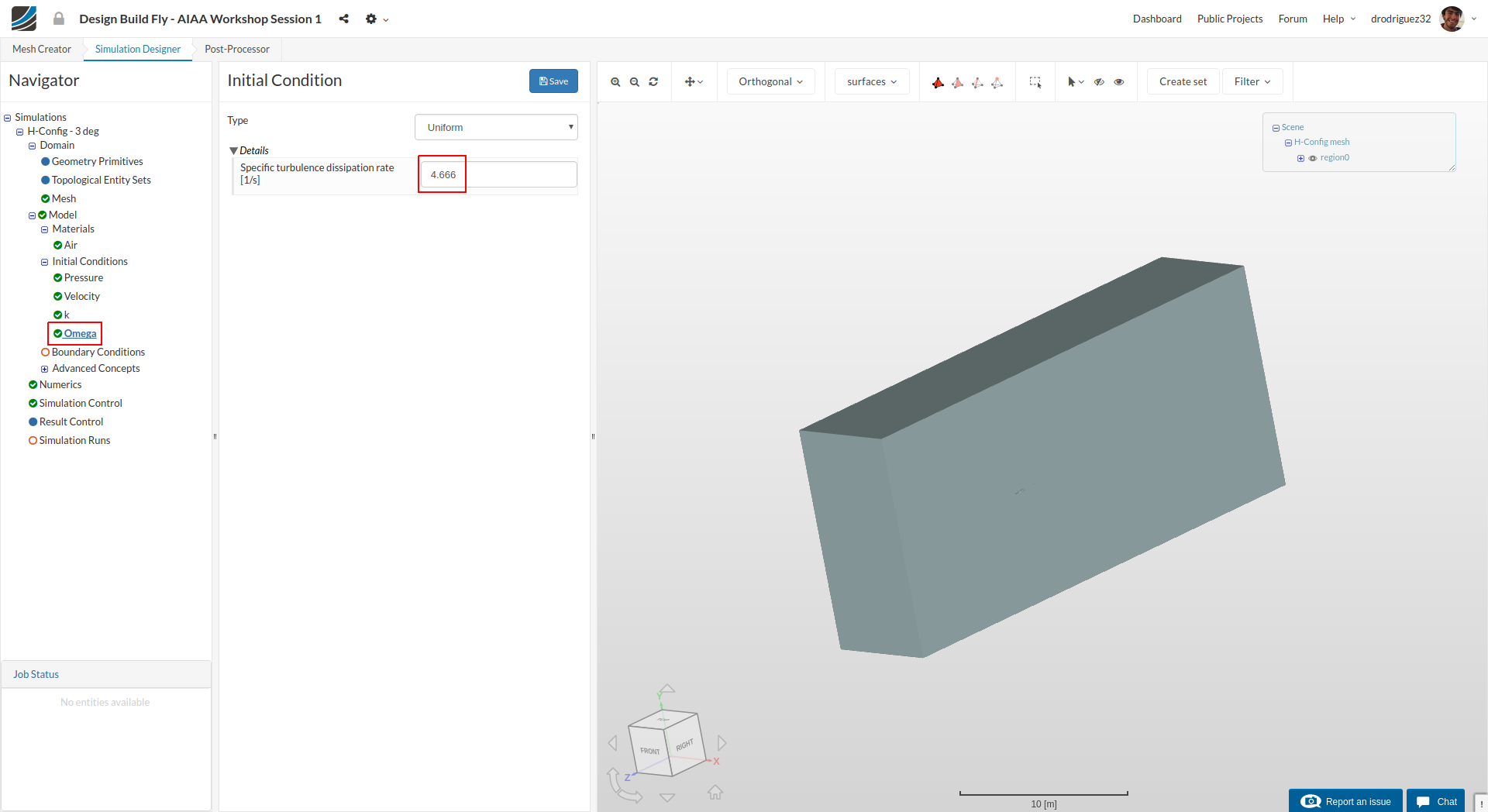
Next go to Omega and change Specific turbulence dissipation rate [1/s] to 4.666 and click Save
The two settings you just modified are associated to the turbulence model that will be applied to this simulation (K-Omega SST). Turbulence is a highly complex process with irregular, chaotic, and unsteady 3D phenomenon. We would need an extremely fine mesh and a huge amount of computational power to correctly simulate it, so the standard process is to apply a model that mathematically predicts this turbulent behavior.
Boundary Conditions
This is one of the most important parts of the simulation set-up. Boundary conditions are how we tell the platform how each thing behaves. So for example where does the air go in and where does it go out? With what speed does the air go into the domain and in what direction? Is the air being slowed down by something (like the wing)? This is what you’ll do now.

Go to Boundary Conditions and click +New in order to create a new boundary condition.
1. Inlet
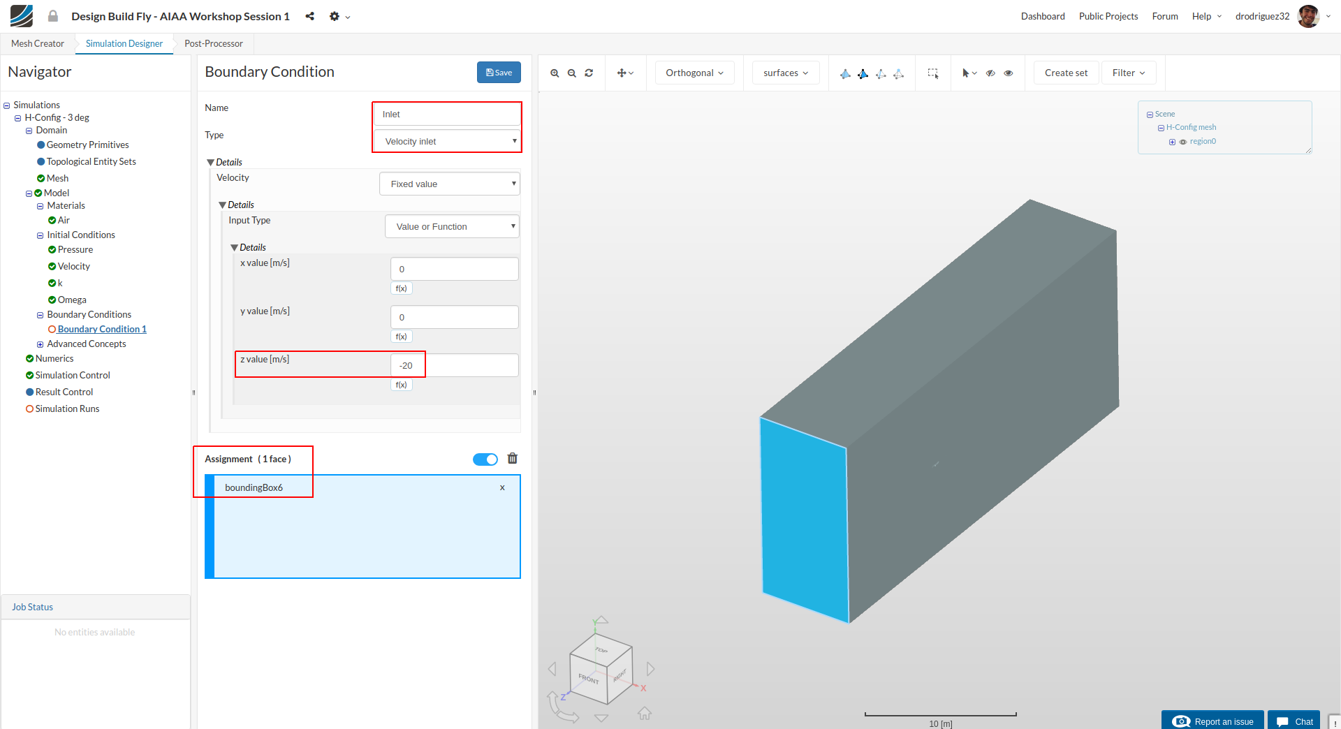
Rename the newly created boundary condition to Inlet (optional).
Make sure that the Type is Velocity Inlet and that under Velocity it says Fixed value. Change the z value [m/s] to -20
Select the front surface of the domain from the viewer and under Assignment you should see boundingBox6.
Click Save to define the inlet boundary condition.
2. Outlet

Create a new Boundary Condition and name it Outlet (optional).
Change Type to Pressure Outlet and select the back surface of the domain. Under Assignment you should see boundingBox5.
Click Save to define the outlet boundary condition.
3. Sides
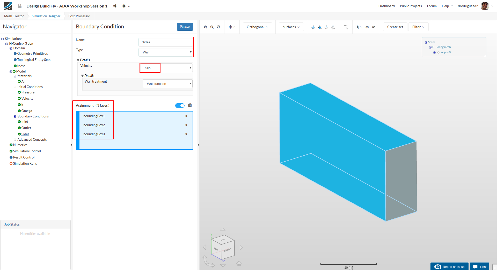
Create a new Boundary Condition and name it Sides (optional).
Change Type to Wall and Velocity to Slip.
Select the side face that doesn’t intersect the plane, and the upper and lower faces. Under Assignment you should see boundingBox1, boundingBox2, and boundingBox3.
Click Save to define the boundary condition for the sides.
4. Symmetry
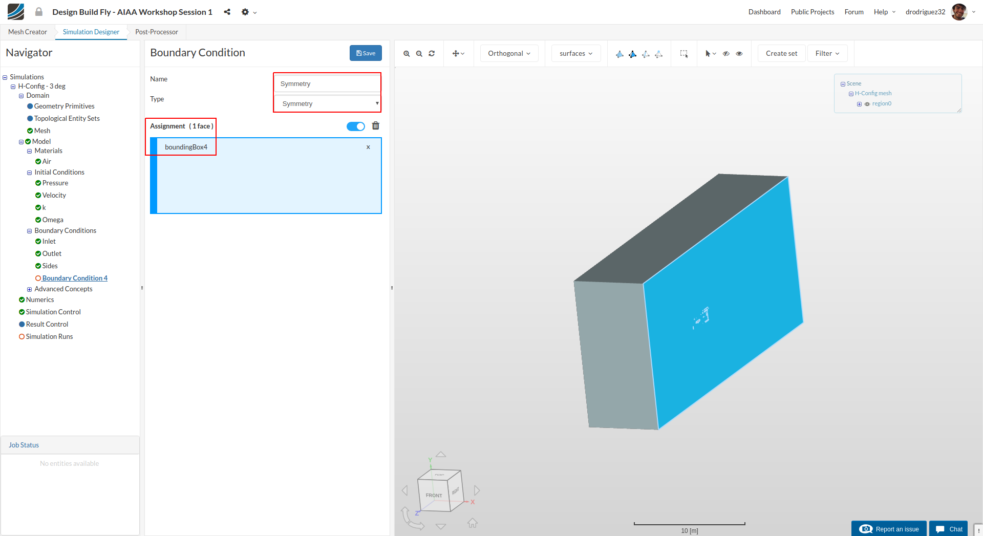
Next we will define the symmetry condition. This is what tells the simulation that in reality we are running a complete airplane. Create a new Boundary Condition and name it Symmetry (optional).
Change Type to Symmetry and select the side face on the inner side of the wing (where it was cut) (boundingBox4).
Click Save to define the symmetry boundary condition.
5. Plane
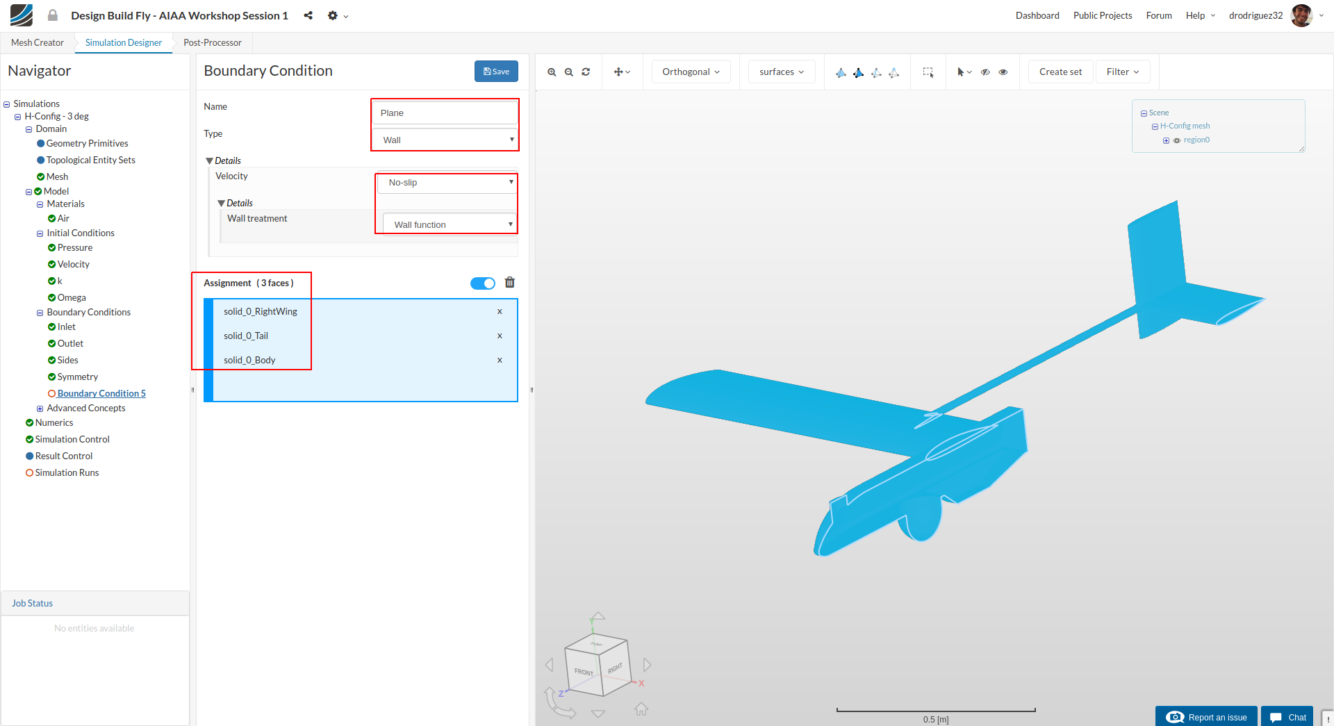
Finally, we will define the boundary condition for the plane. Create a new boundary condition and rename it to Plane (optional).
Change Type to Wall and Velocity to No-slip. Also, make sure under Wall treatment it says Wall function.
With this No-slip condition you are specifying that there is friction between the plane and the air and thus a boundary layer will be formed.
Make sure you hide the bounding box by using the navigator on the right. Select all the faces. Under Assignment you should see solid_0_RightWing, solid_0_Tail, and solid_0_Body.
Click Save to define the boundary condition for the wing.
Numerics
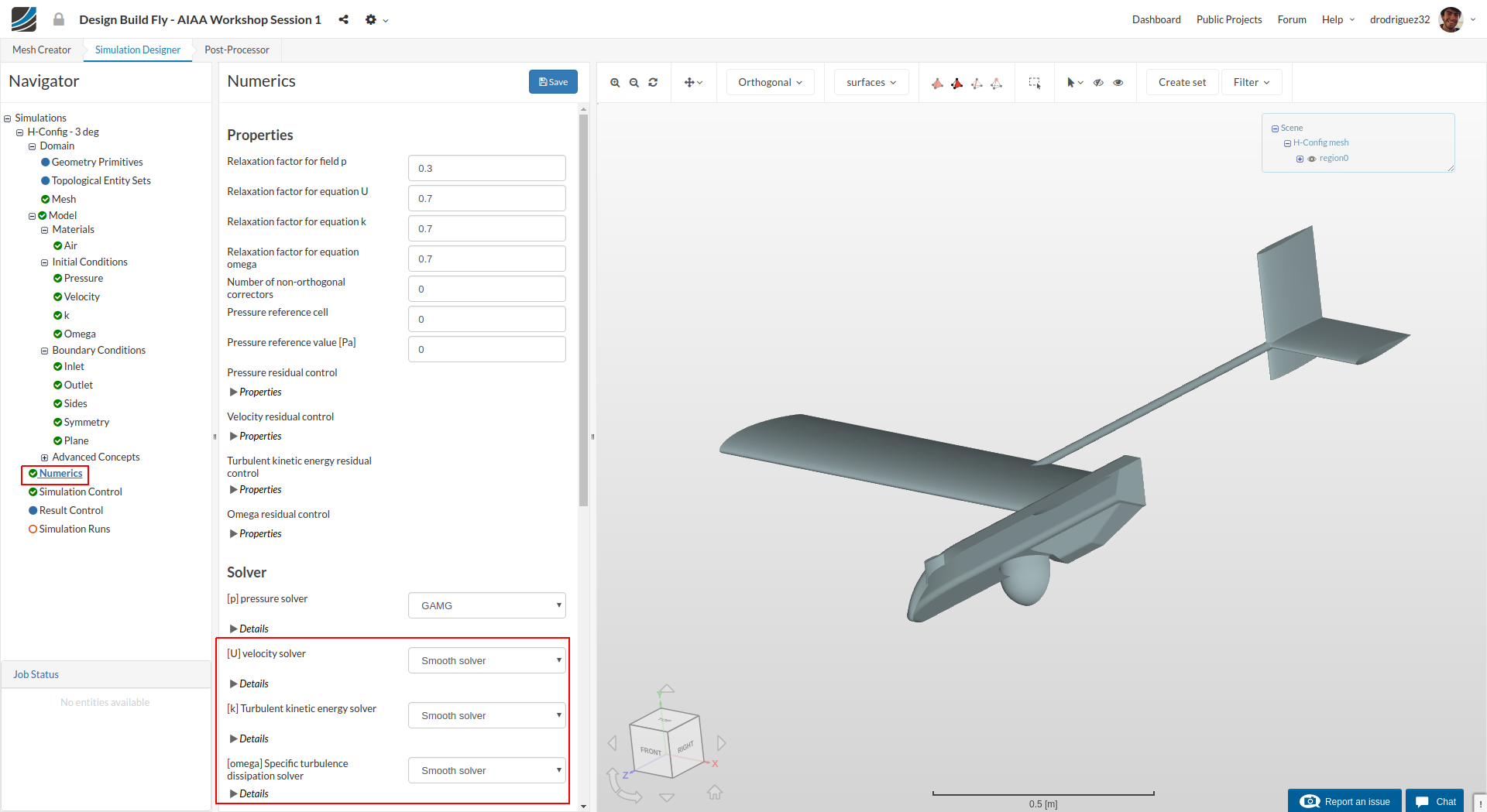
After defining all the boundary conditions, we will proceed to set up the numerics for our simulation. Go to Numerics and scroll down until you reach Solver.
Under Solver, change [U] velocity solver, [k] Turbulent kinetic energy solver, and [omega] Specific turbulence dissipation solverto Smooth solver.
Click Save to register your changes.
Simulation Control
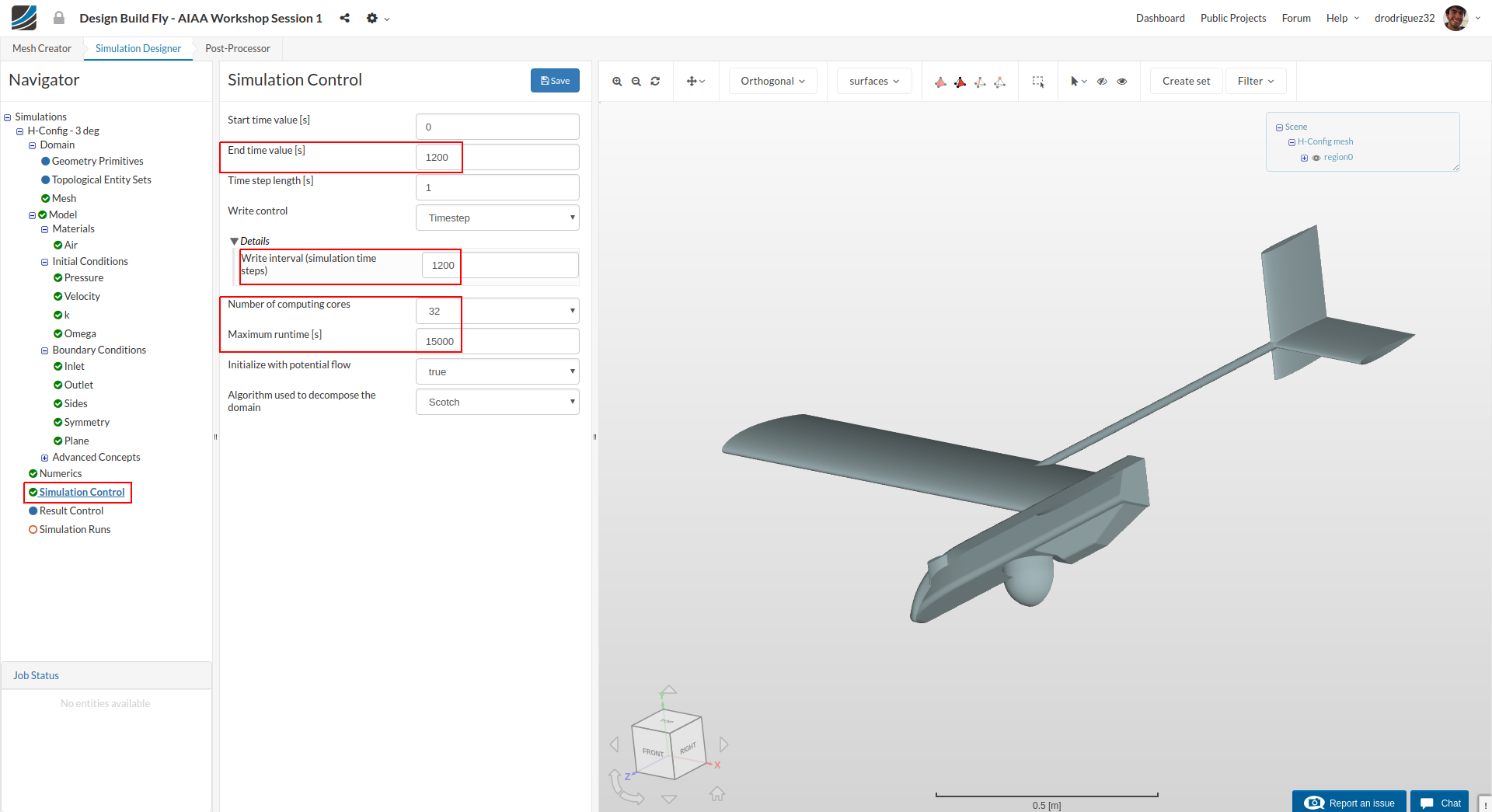
Next we will define the our simulation interval and steps that needs to be recorded. Go to Simulation Control and change End time value [s] to 1200.
Expand Details under Write control and change Write interval (simulation time steps) to 1200.
Next change Number of computing cores and Maximum runtime [s] to 32 and 15,000 respectively. The Maximum runtime [s] is a safety feature that will cut your simulation if it exceeds that time in order to save core hours.
Click Save to register your changes.
Result Control
As our last step before running the simulation, we will create result control items in order to get graphical data sets of interest. These control items allow us to see when a simulation has reached steady state (when forces become constant) and it also lets us see things like the lift and drag of the wing.
Forces & Moments

Go to Result Control in the navigator. We will create the result control item for the forces and moments. Click New next to Forces and Moments.
1. Wing
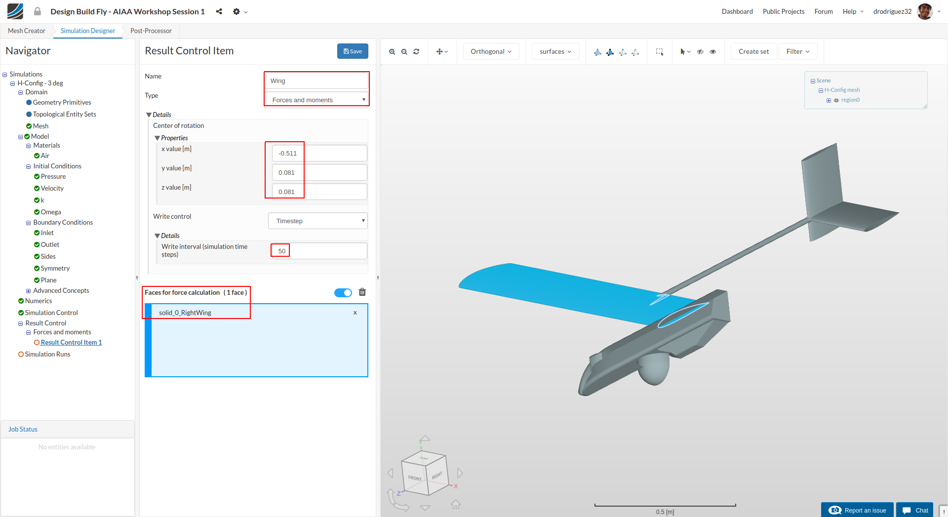
A new force and moment result control item will be created. Rename it to Wing (optional).
Change the center of rotation to the center of gravity of the object.
- x value: -0.511
- y value: 0.081
- z value: -0.122
Select the main wing and under Faces for force calculation you should see solid_0_RightWing.
Change the Write Interval to 50. This will save the information for the result control items every 50 time steps and thus will help us save some computation time (as we don’t need to save every single time step).
Lift & Drag
To correctly calculate the lift and drag coefficients in SimScale, we have to put in a bit extra work. As you know, each of those coefficients requires a reference area for calculation. For this we need the plan area of the wing:
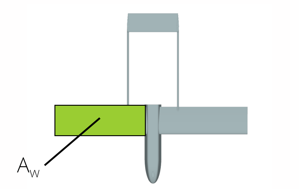
In your CAD tool, you can create two planes (one parallel and one perpendicular to the flow), and project the area of the wing onto those planes.
Wing CL
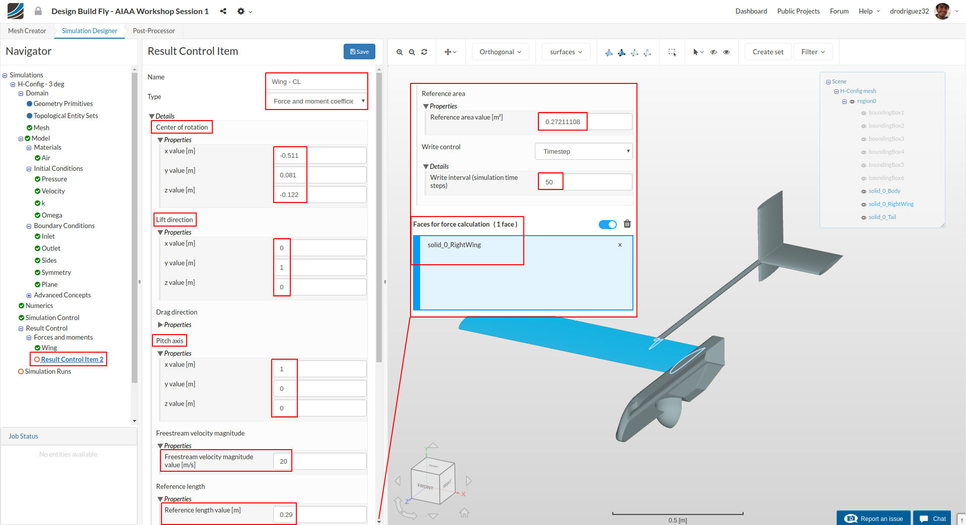
Create a new Result Control Item and rename it to “Wing - CL” (optional).
Under Type select Force and moment coefficients and change the following values:
-
Center of Rotation - should be the center of gravity of the object
a. x value: -0.511
b. y value: 0.081
c. z value: -0.122 -
Lift direction - the vector that describes the direction in which lift is acting.
a. Just change the y value to 1 making your vector (0, 1, 0). -
Drag Direction - because we are concerned with lift in this result control item, don’t change anything for this setting
-
Pitch axis
a. Change the x value to 1 -
Freestream velocity
a. Change it to 20 which is the speed at which the plane is travelling -
Reference length - this is the chord length of the wing
a. Change to 0.29 -
Reference area - this is the area that you projected to a plane parallel to the flow direction
a. Change to 0.27211108 -
Write control - this specifies how many times should this result be written to the solution. We don’t need it to be saved every step so change it to 50
Select the wing (solid_0_RightWing).
Click Save to save your changes.
Wing CD
Now we will calculate the drag coefficient
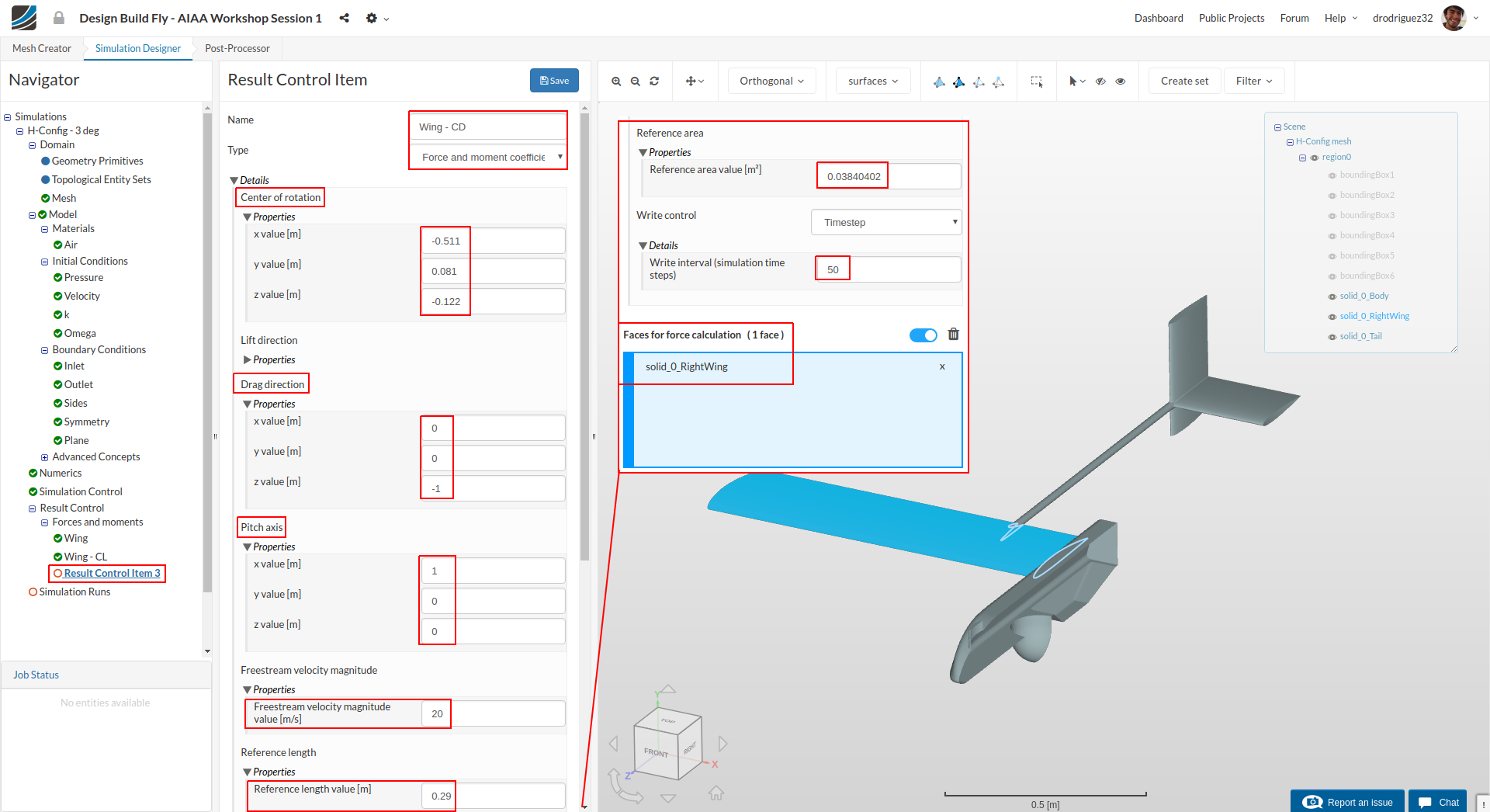
Create a new Result Control Item and rename it to “Wing - CD” (optional).
Under Type select Force and moment coefficients and change the following values:
-
Center of Rotation - should be the center of gravity of the object
a. x value: -0.511
b. y value: 0.081
c. z value: -0.122 -
Lift direction - because we are concerned with drag in this result control item, don’t change anything for this setting
-
Drag Direction - the vector that describes the direction in which drag is acting.
a. Just change the z value to -1 making your vector (0, 0, -1). -
Pitch axis
a. Change the x value to 1 -
Freestream velocity
a. Change it to 20 which is the speed at which the plane is travelling -
Reference length - this is the chord length of the wing
a. Change to 0.29 -
Reference area - this is the area that you projected to a plane perpendicular to the flow direction
a. Change to 0.27211108 -
Write control - this specifies how many times should this result be written to the solution. We don’t need it to be saved every step so change it to 50
Select the wing (solid_0_RightWing).
Click Save to save your changes.
Field Calculations
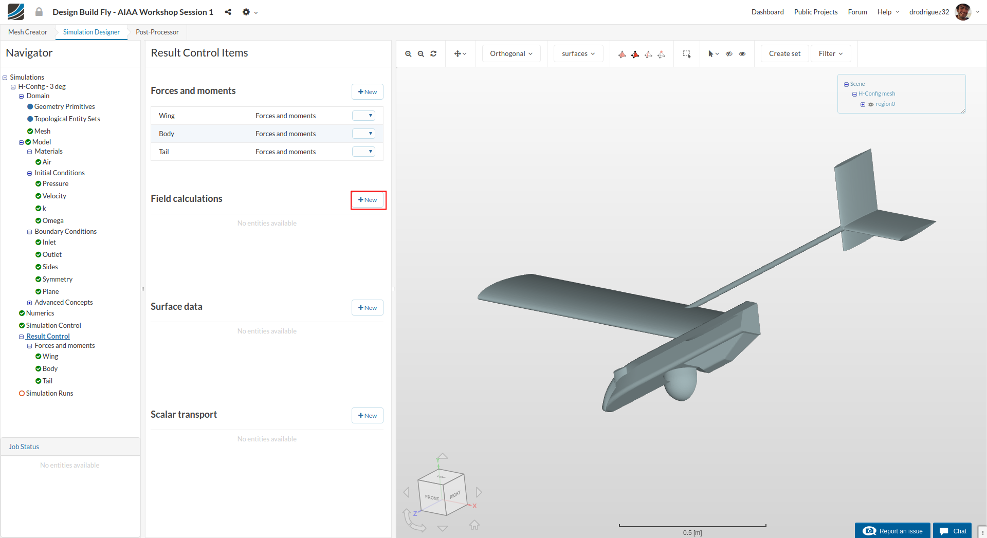
Next, we will create the field calculation items. For this go back to Result Control and click New next to Field calculations.
Y-Plus
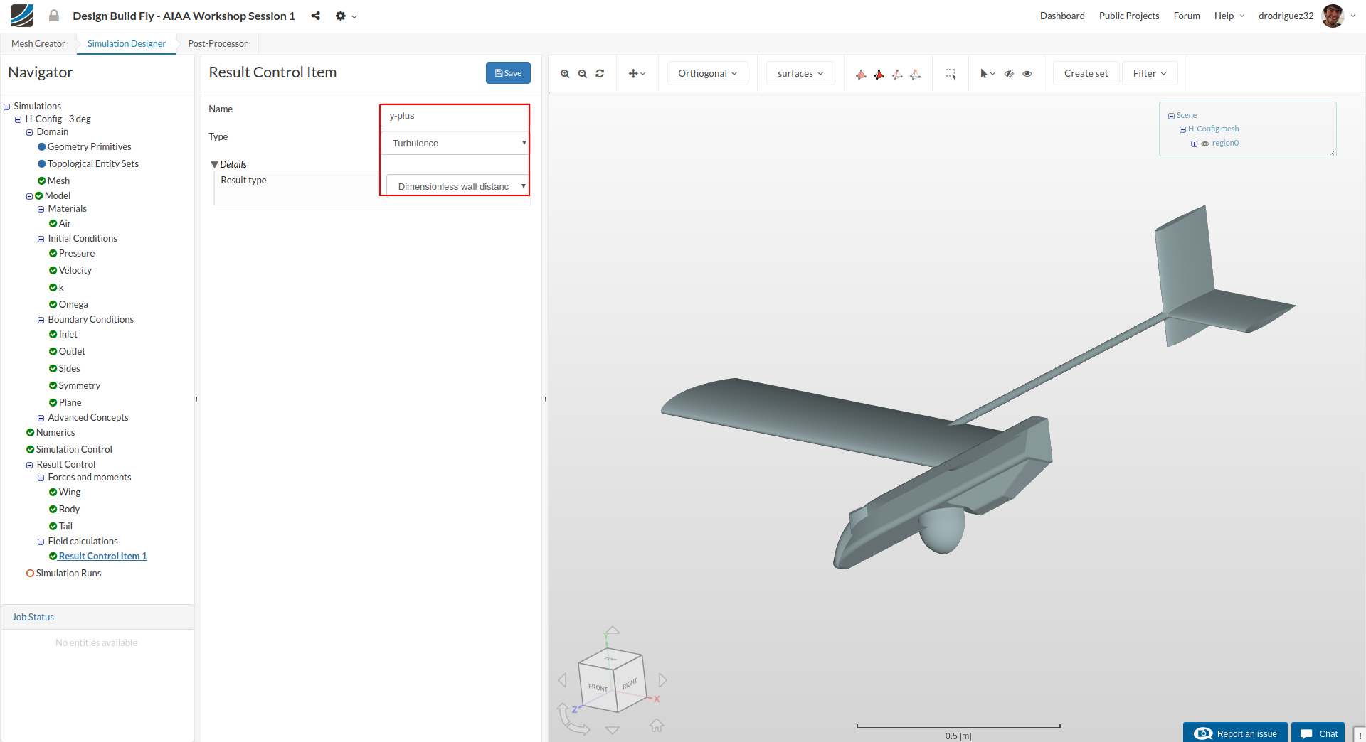
Rename the newly created field calculation item to Yplus (optional).
Change the Type to Turbulence and click Save to register your changes.
Wall Shear Stress
Create another field calculation item and rename it to WallShearStress (optional).
Change the Type to Wall fluxes and click Save to register your changes.
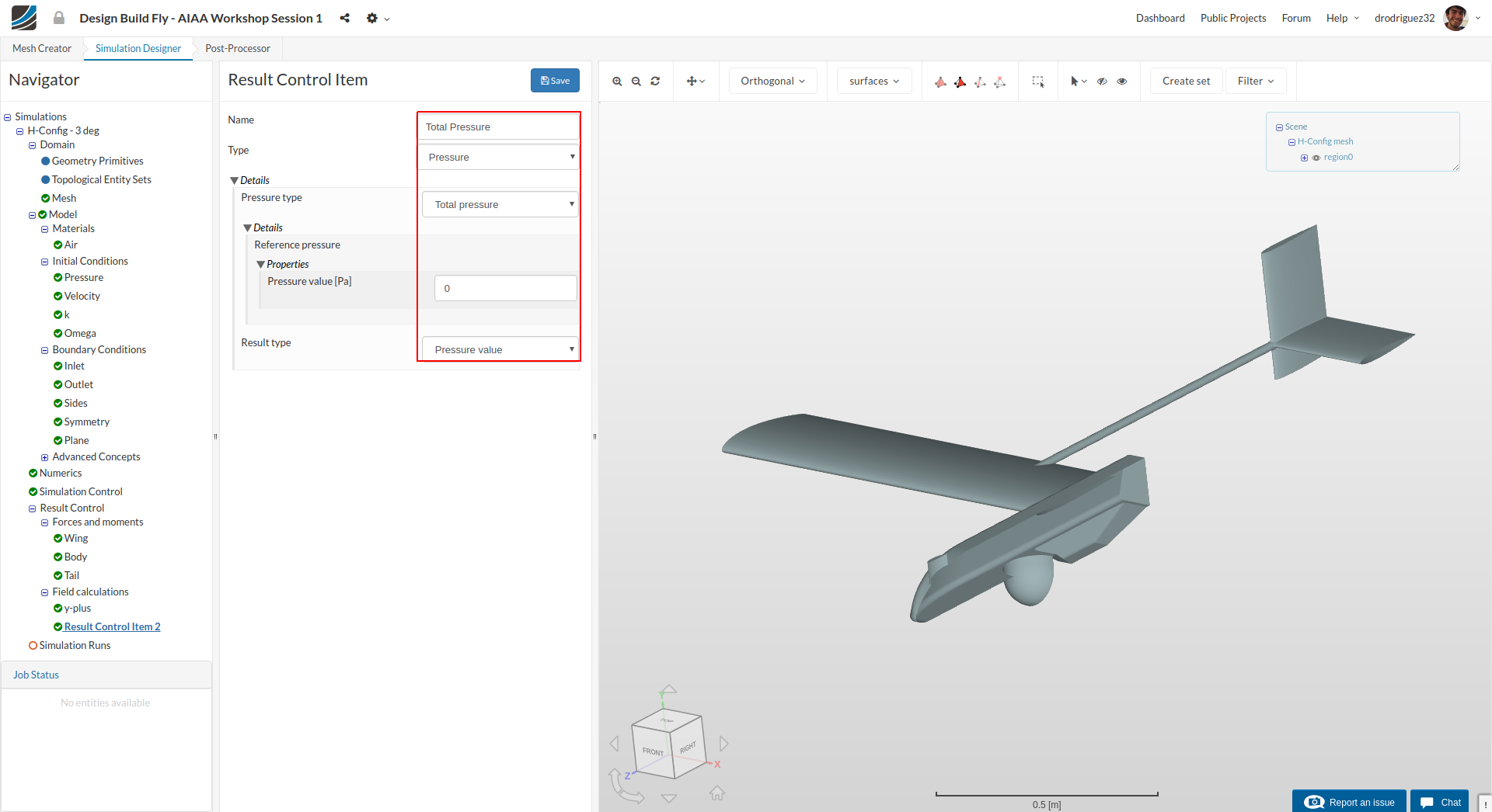
Surface Data
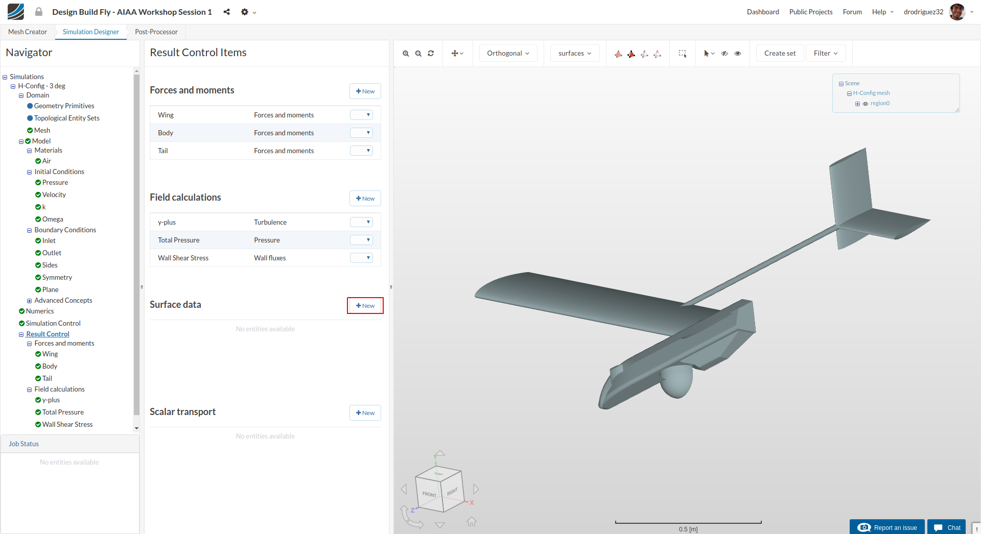
Finally, we will create a Surface Data item. For this go back to Result Control and click New next to Surface data.
Outlet
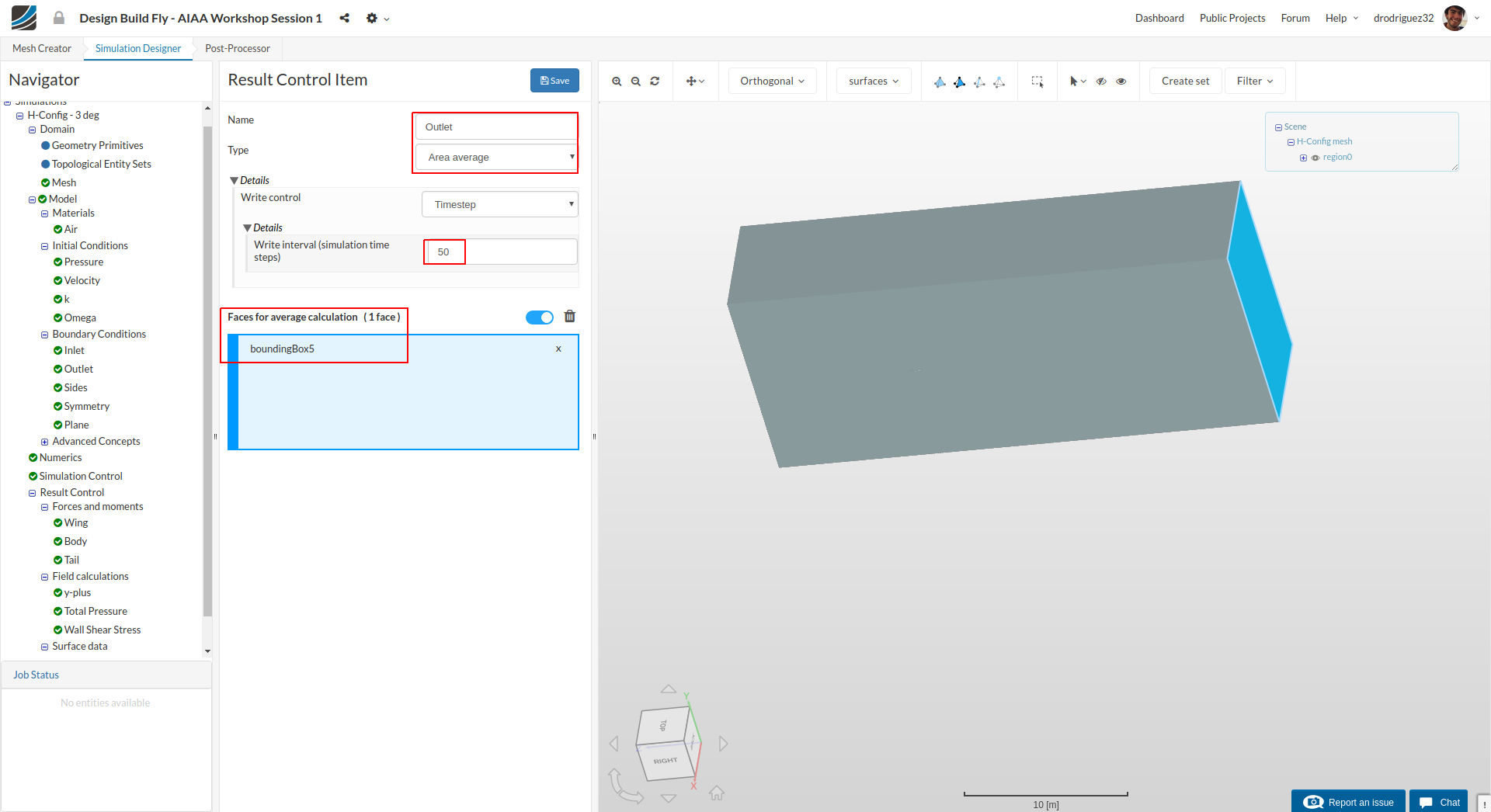
Rename the newly created item to “Outlet” (optional), select the outlet of the domain (boundingBox5), and change Write interval to 50.
Simulation Runs
Once all the above steps are defined, we will proceed to create our first simulation run.
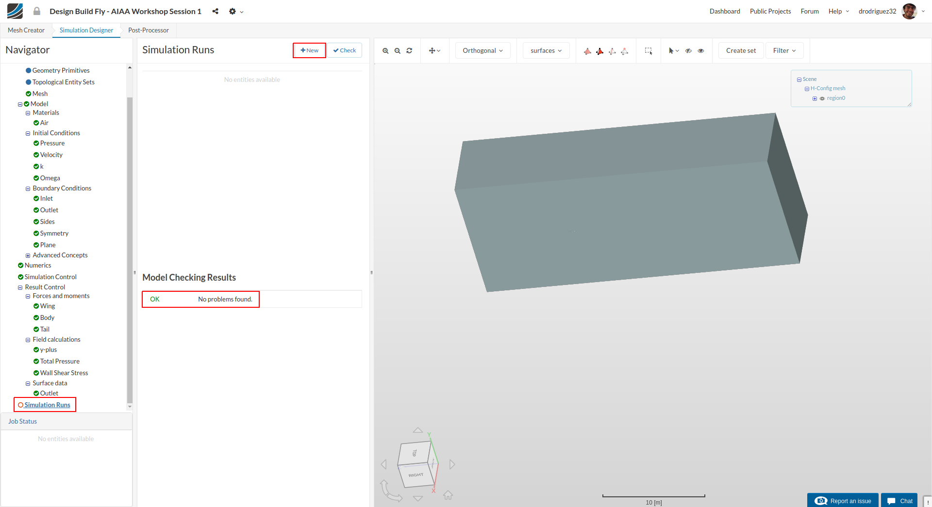
Go to Simulation Runs and click on New.
A window will pop up, give a reasonable name to the run e.g. Run-3deg in this case (optional) and click Start to initialize this run. The simulation run can around 180 minutes (~3 hrs.).
Recommendations About Comments
If you run into issues during your process, before adding a comment to the thread please consider the following:
- Go over the tutorial one last time and compare it to your setup. Is everything the same?
- Go over the existing comments. Maybe someone has had the same problem and it’s already solved.
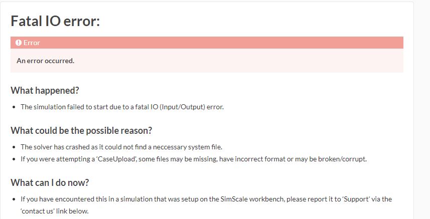
- Is there an actual error? Or is it taking a long time to load?
a. If it seems to be a loading issue, please give it some time or refresh the page. Sometimes due to the internet connection the platform may seem slow.
If it’s a new issue that you can’t solve, please outline the issue as specifically as possible and include a link to your project. This will help us figure out what is going on faster and thus we can get back to you faster.
Continue to part 2 of the tutorial:
DBF Workshop Session 1 - Aerodynamic Study of Model Plane (Part 2)