Link to part 1 of the tutorial:
DBF Workshop Session 1 - Aerodynamic Study of Model Plane (Part 1)
Introduction
Welcome to the second part of the step-by-step tutorial for the simulation of a model airplane. In this part of the tutorial we will show you how to setup a simulation to investigate different angles of attack without changing the mesh.
Simulation Setup for Different AOA
Now we will go through the setup of the simulation for the modified angle of attack. It doesn’t involve as many steps as before! We will just modify some of the boundary conditions.
Duplicating a Simulation
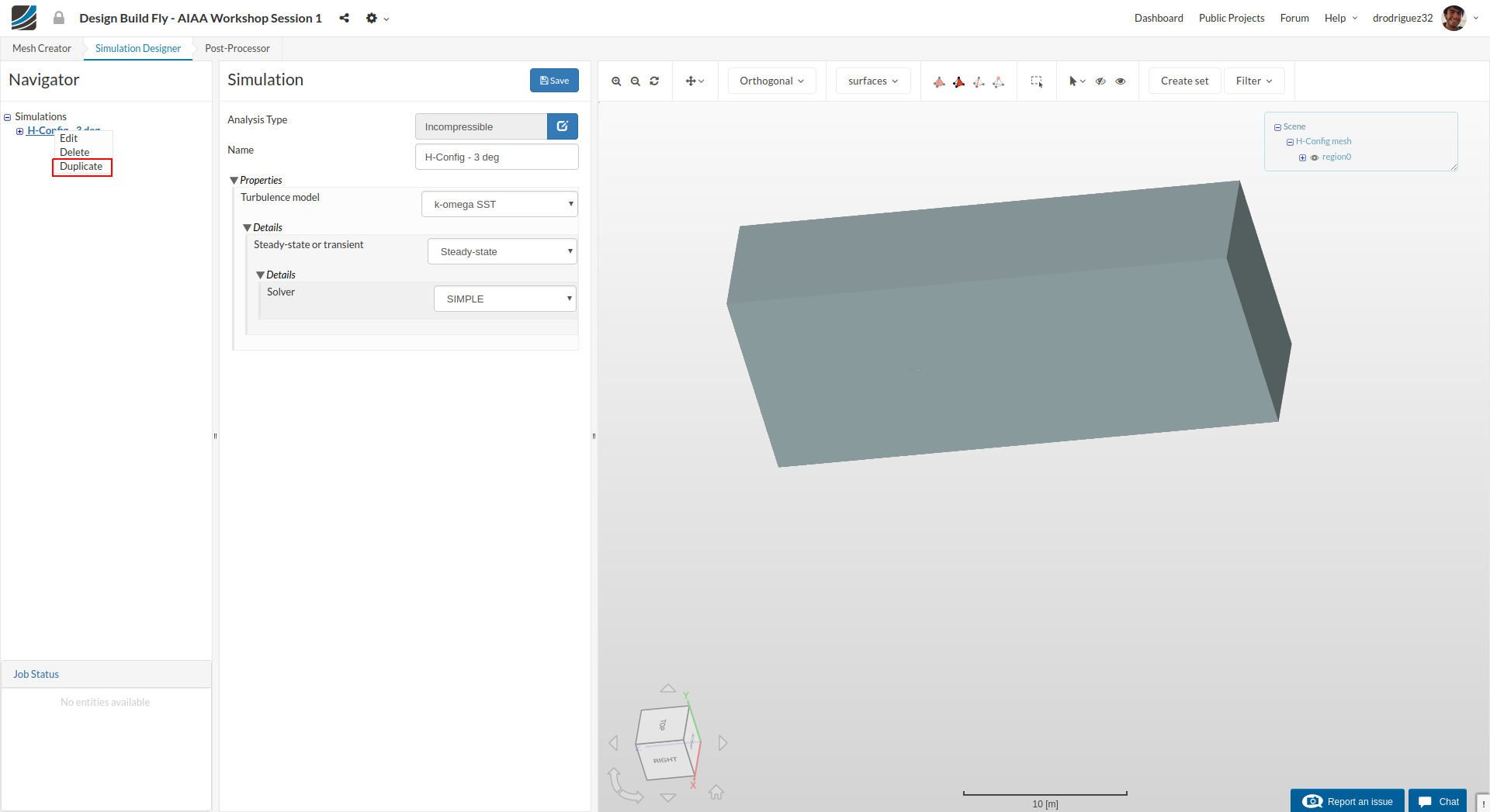
Right click on your simulation, and click on Duplicate. This will create a copy of the simulation we just set up.

Rename your simulation to “H-Config - 20 deg” (optional) and click save.
Boundary Conditions
In order to save time and computational capacity, we don’t want to use two different models and two different meshes to see the effects of a different angle of attack. So how do we change the angle of attack without changing the model? We can simply change the angle of incidence of the air, which will lead to a different angle of attack.
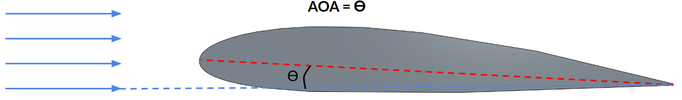
Here you can see that the AOA is the angle between the centerline and the flow direction. In this case, air is moving straight past the wing with no incidence angle, and as such the AOA is simply theta. This is the first simulation we did.
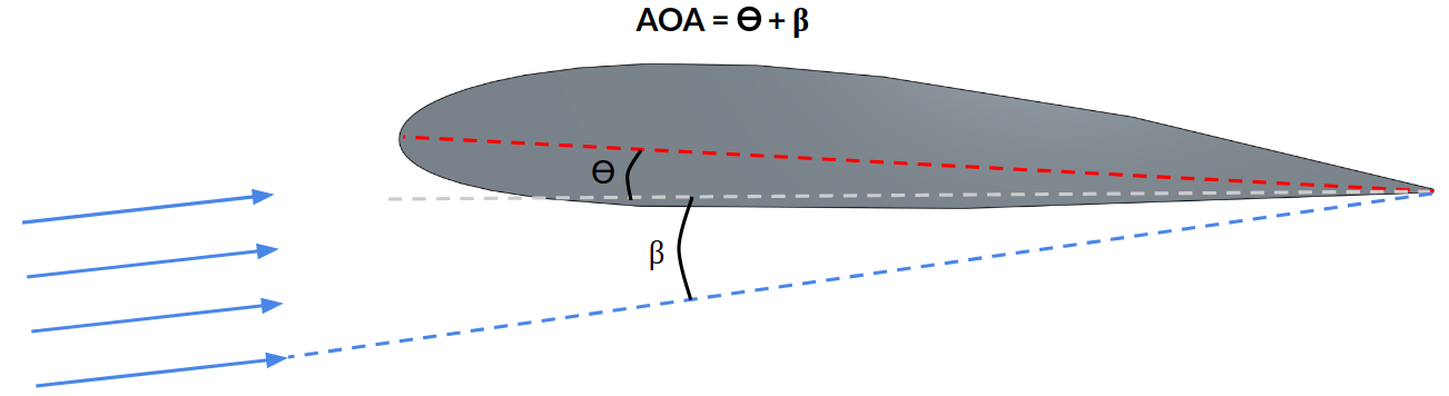
But here, the air has an angle of incidence beta, and as such, the AOA for this wing becomes theta + beta. This is exactly what we will do within the boundary conditions.
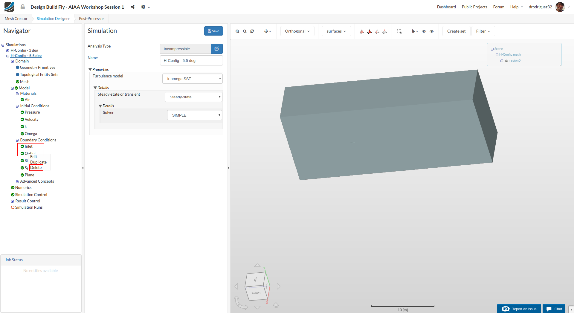
First, go to the boundary conditions, right click on Inlet and select Delete. Do the same for Outlet.
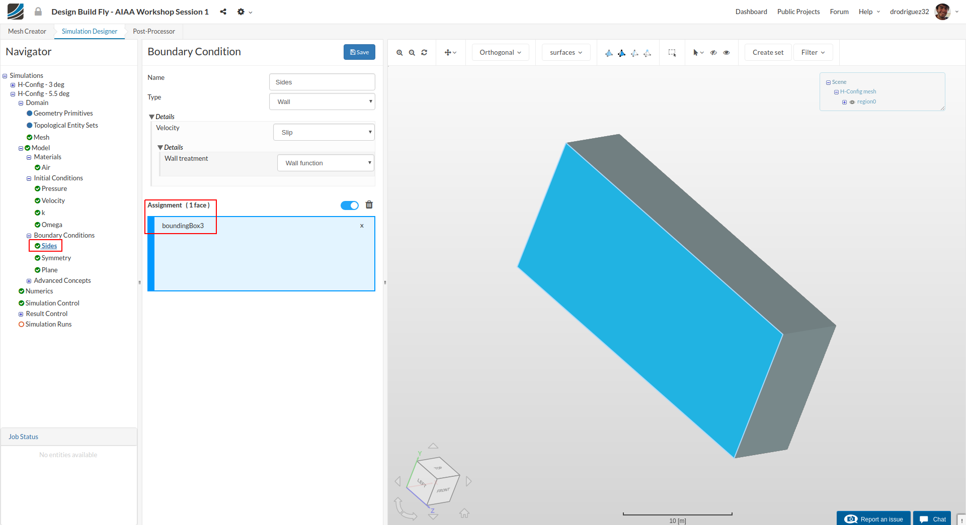
Next, go to the Sides boundary condition and remove all the faces except bundingBox3. This will remain as a normal slip wall.
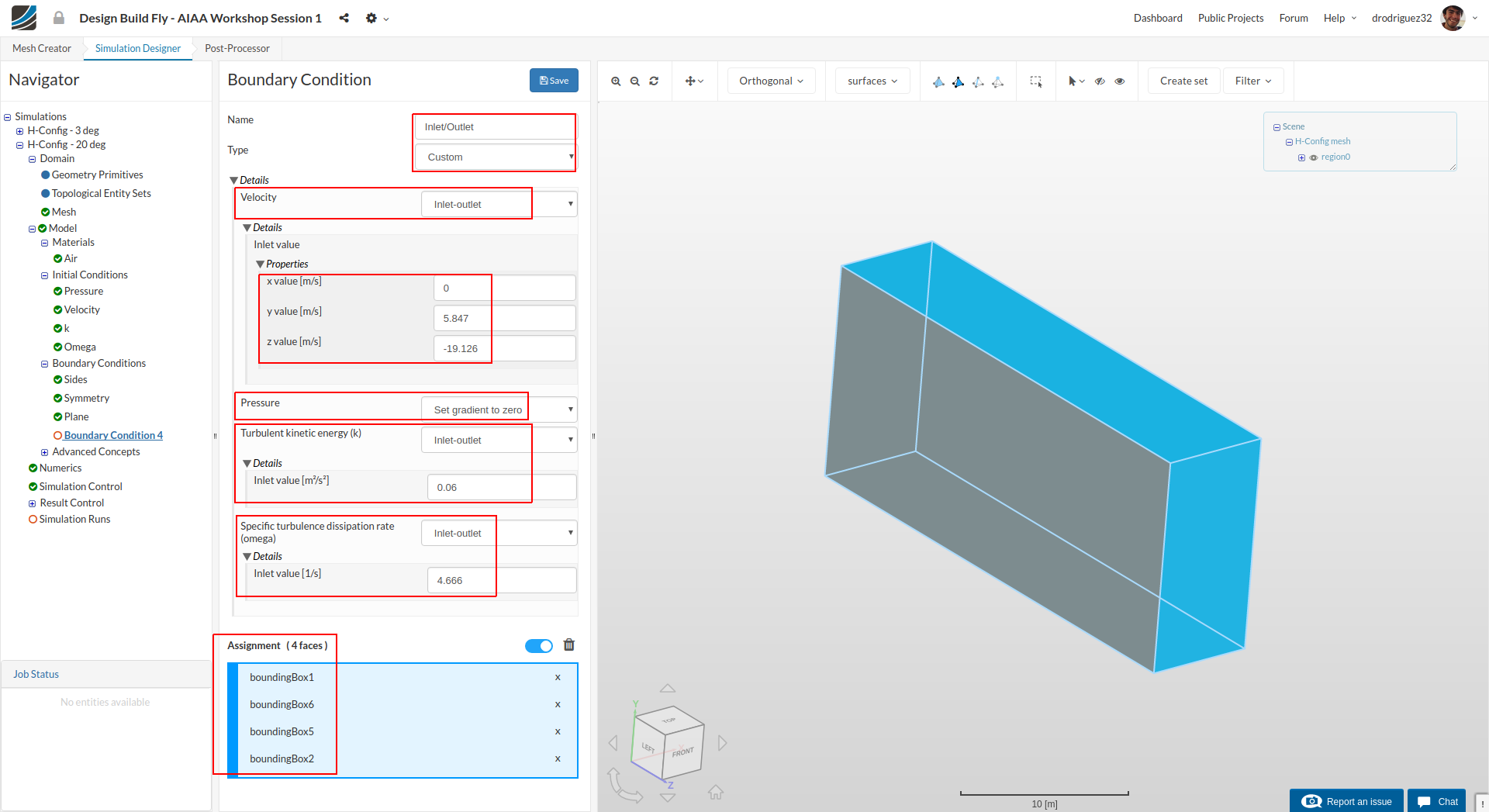
Create a new boundary condition and rename it to “Inlet/Outlet” (optional).
Change the Type to Custom, and do the following:
- Velocity: Inlet-outlet
a. x value: 0
b. y value: 5.847
c. z value: -19.126
Here we just defined that air is moving at 20 m/s with an angle of 17 degrees from the horizontal plane (this would be beta in the above diagrams). When you add it to the original angle of attack (theta = 3 degrees) you get AOA = 20 degrees.
-
Pressure: Set gradient to zero
-
Turbulent kinetic energy (k): Inlet-outlet
a. Inlet value: 0.06 -
Specific turbulence dissipation rate (omega): Inlet-outlet
a. Inlet value: 4.666 -
Select boundingBox1, boundingBox2, boundingBox5, and boundingBox6.
Click Save
Lift & Drag
Wing CL
Now we’re going to adjust the result control items so that they match the new angle of attack/angle of incidence.
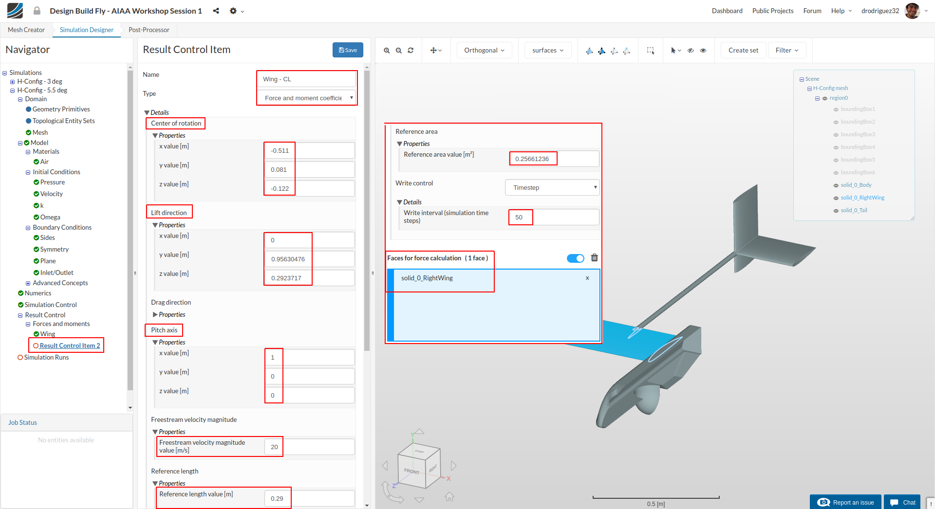
Go to Wing - CL
Under Type select Force and moment coefficients and change the following values:
-
Center of Rotation - should be the center of gravity of the object
a. x value: -0.511
b. y value: 0.081
c. z value: -0.122 -
Lift direction - the vector that describes the direction in which lift is acting (perpendicular to the flow direction).
a. x value: 0
b. y value: 0.95630476
c. z value: 0.2923717 -
Drag Direction - because we are concerned with lift in this result control item, don’t change anything for this setting
-
Pitch axis
a. Change the x value to 1 -
Freestream velocity
a. Change it to 20 which is the speed at which the plane is travelling -
Reference length - this is the chord length of the wing
a. Change to 0.29 -
Reference area - this is the area that you projected to a plane parallel to the flow direction
a. Change to 0.27211108 -
Write control - this specifies how many times should this result be written to the solution. We don’t need it to be saved every step so change it to 50
Select the wing (solid_0_RightWing).
Click Save to save your changes.
Wing - CD
Now we will calculate the drag coefficient
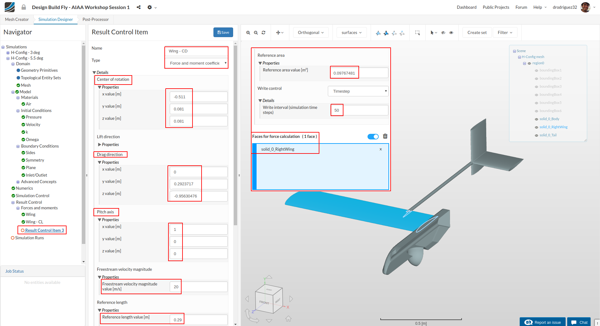
Go to Wing - CD
Under Type select Force and moment coefficients and change the following values:
-
Center of Rotation - should be the center of gravity of the object
a. x value: -0.511
b. y value: 0.081
c. z value: -0.122 -
Lift direction - because we are concerned with drag in this result control item, don’t change anything for this setting
-
Drag Direction - the vector that describes the direction in which drag is acting.
a. x value: 0
b. y value: 0.2923717
c. z value: -0.95630476 -
Pitch axis
a. Change the x value to 1 -
Freestream velocity
a. Change it to 20 which is the speed at which the plane is travelling -
Reference length - this is the chord length of the wing
a. Change to 0.29 -
Reference area - this is the area that you projected to a plane perpendicular to the flow direction
a. Change to 0.27211108 -
Write control - this specifies how many times should this result be written to the solution. We don’t need it to be saved every step so change it to 50
Select the wing (solid_0_RightWing).
Click Save to save your changes.
Go to Simulation Runs and run a new simulation for the new angle of attack.
Post-processing
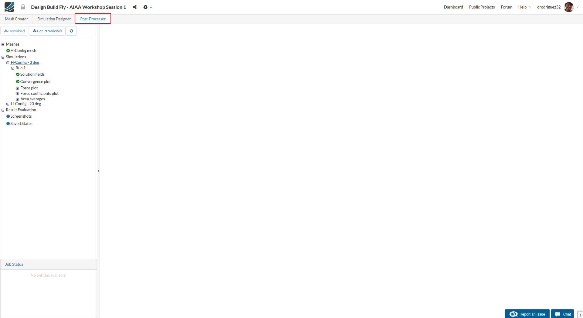
When your simulation is completed, proceed to Post-Processor tab in order to post-process your results.
We will show the post-processing only for the first simulation results. You can then follow the same steps in order to post-process other configuration results
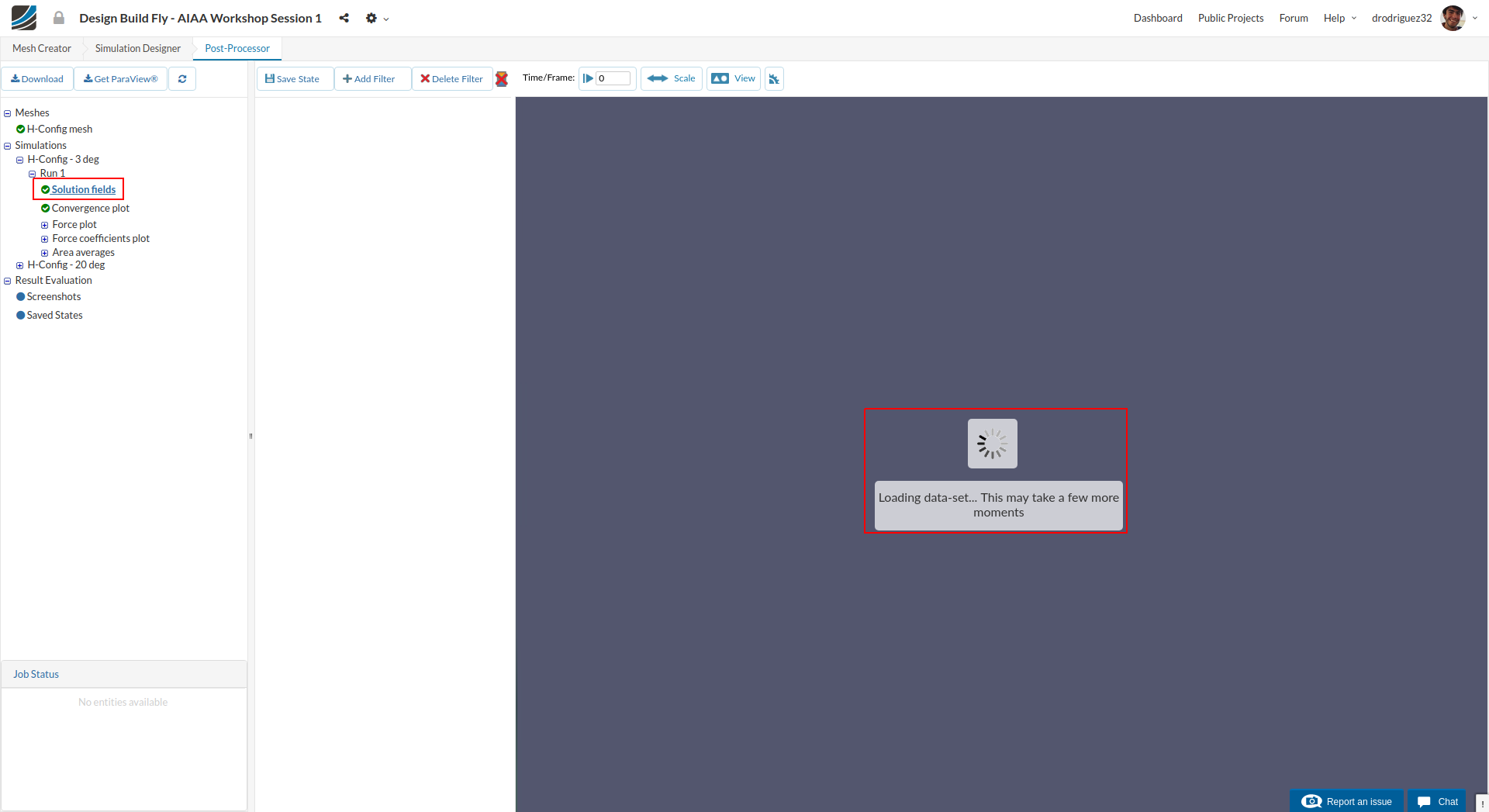
Once in Post-Processor, click on Solution fields under H-Config - 3 deg in order to load the results in the viewer. Due to fine mesh it can take a while to load the results in to the viewer.
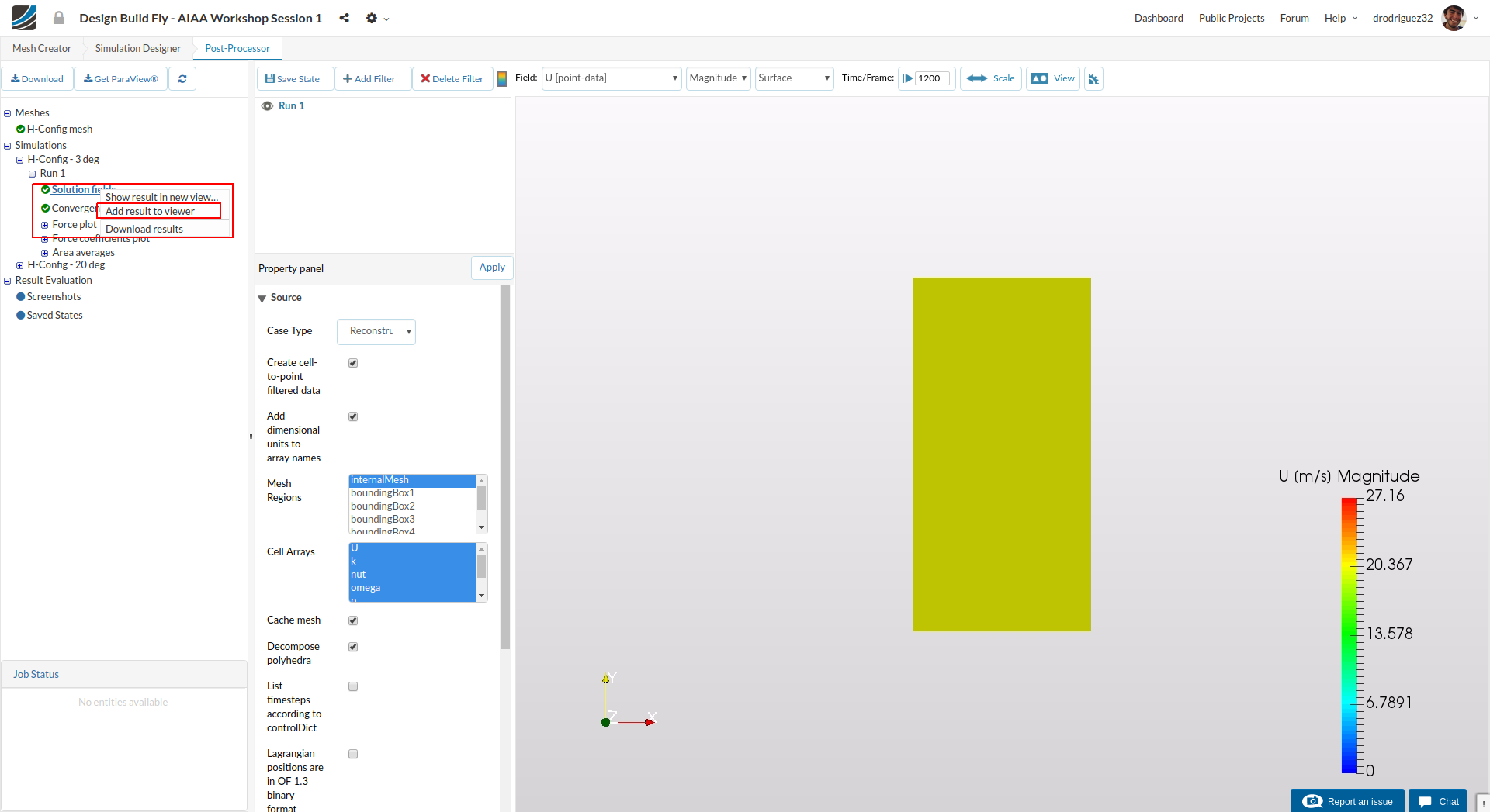
Once the results have loaded, right click on Solution fields and select Add results to viewer - this will also take a while. The first set of results that loaded will be used only for the fluid, and this second set will be used for the surfaces of the plane.
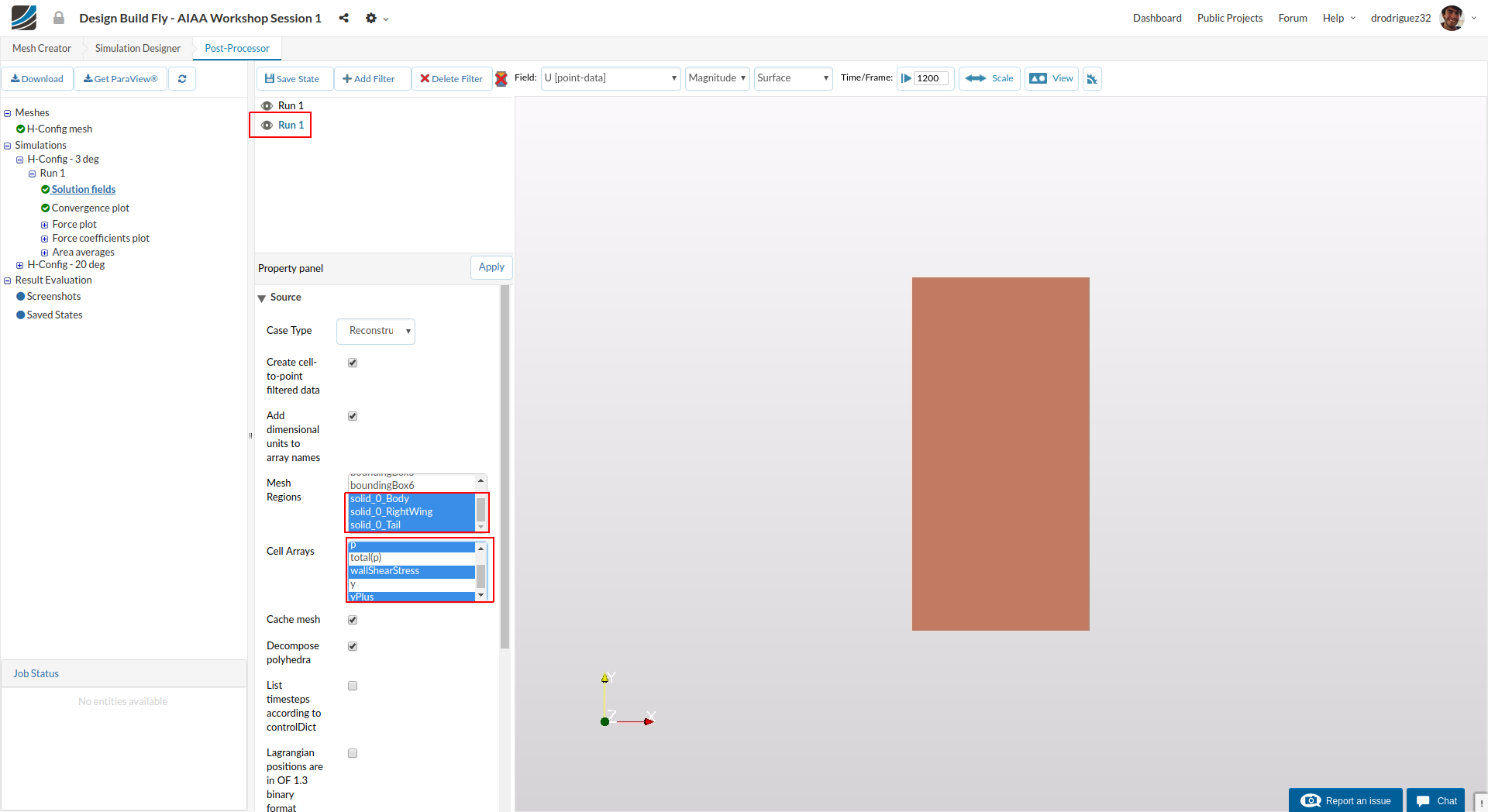
Once the second set has loaded, under Mesh Regions select only the regions that correspond to the surfaces of the plane: solid_0_Body, solid_0_RightWing, and solid_0_Tail. You can select multiple entities using Ctrl + click.
Additionally, under Cell Arrays, select only the following variables: p, wallShearStress, and yPlus. These are the values of greatest interest directly on the surface of the wing.
Click Apply
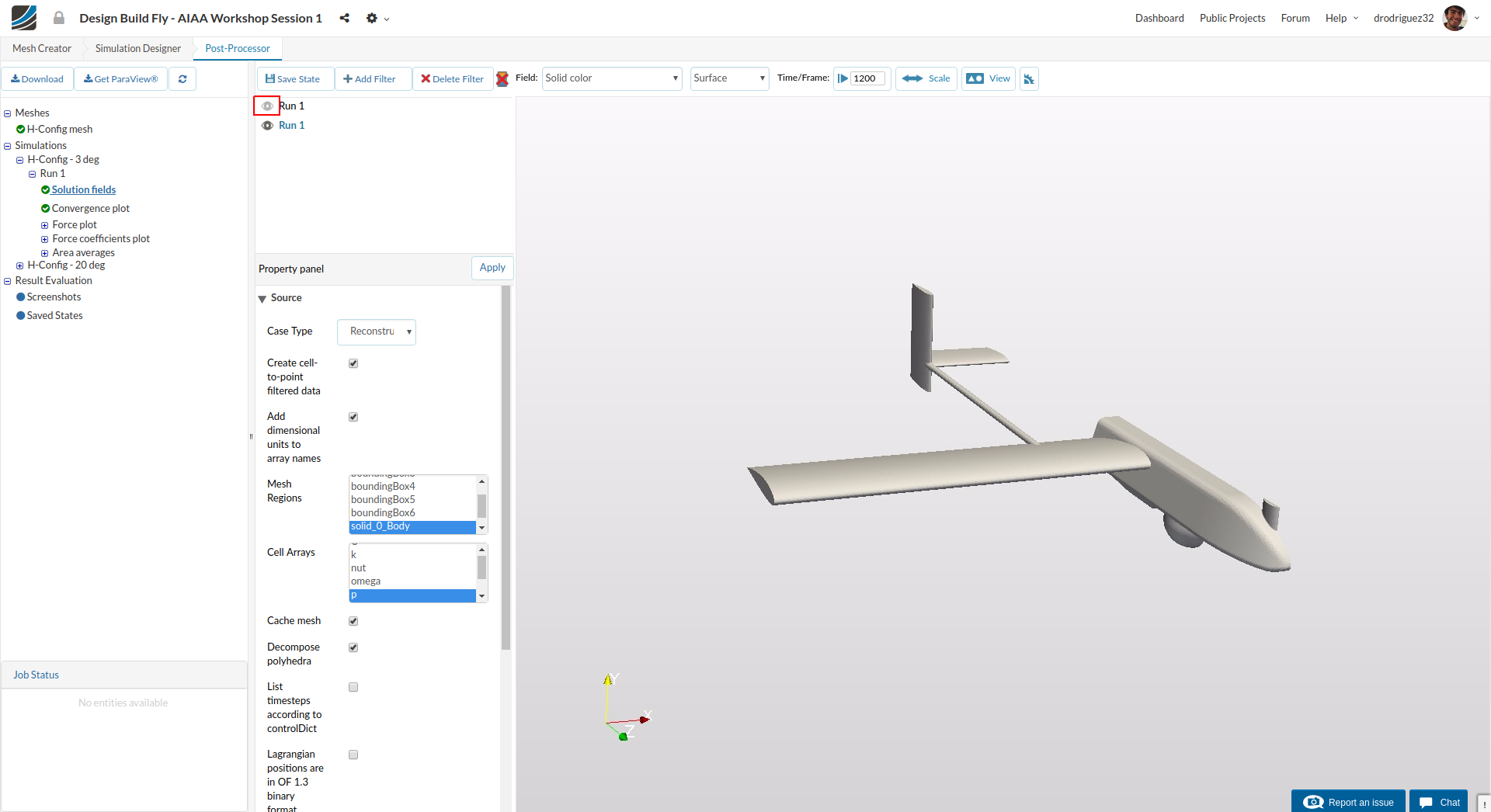
Hide the fluid region by clicking on the small eye to the left of the the first results.
We will now start visualizing the results.
Filters/Visualization
Slice
We will start with adding a slice.
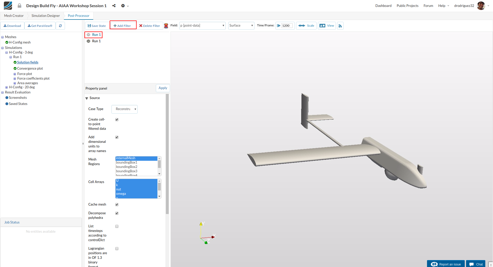
Make sure you click on the first set of results (so that it is highlighted in blue) and then click on Add Filter
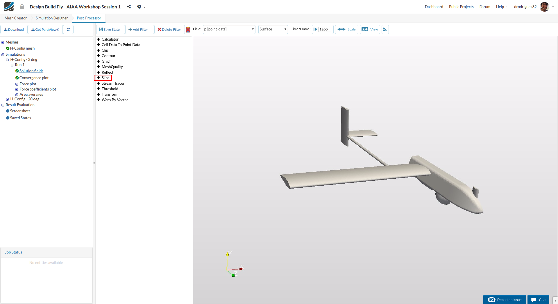
From the list click on Slice
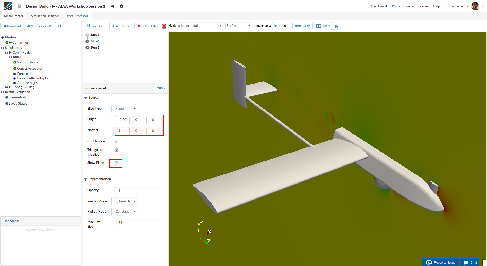
Once it has loaded, change the following:
-
Change Origin to -0.001, 0, 0
-
Uncheck Show Plane.
-
Click Apply to save the changes.
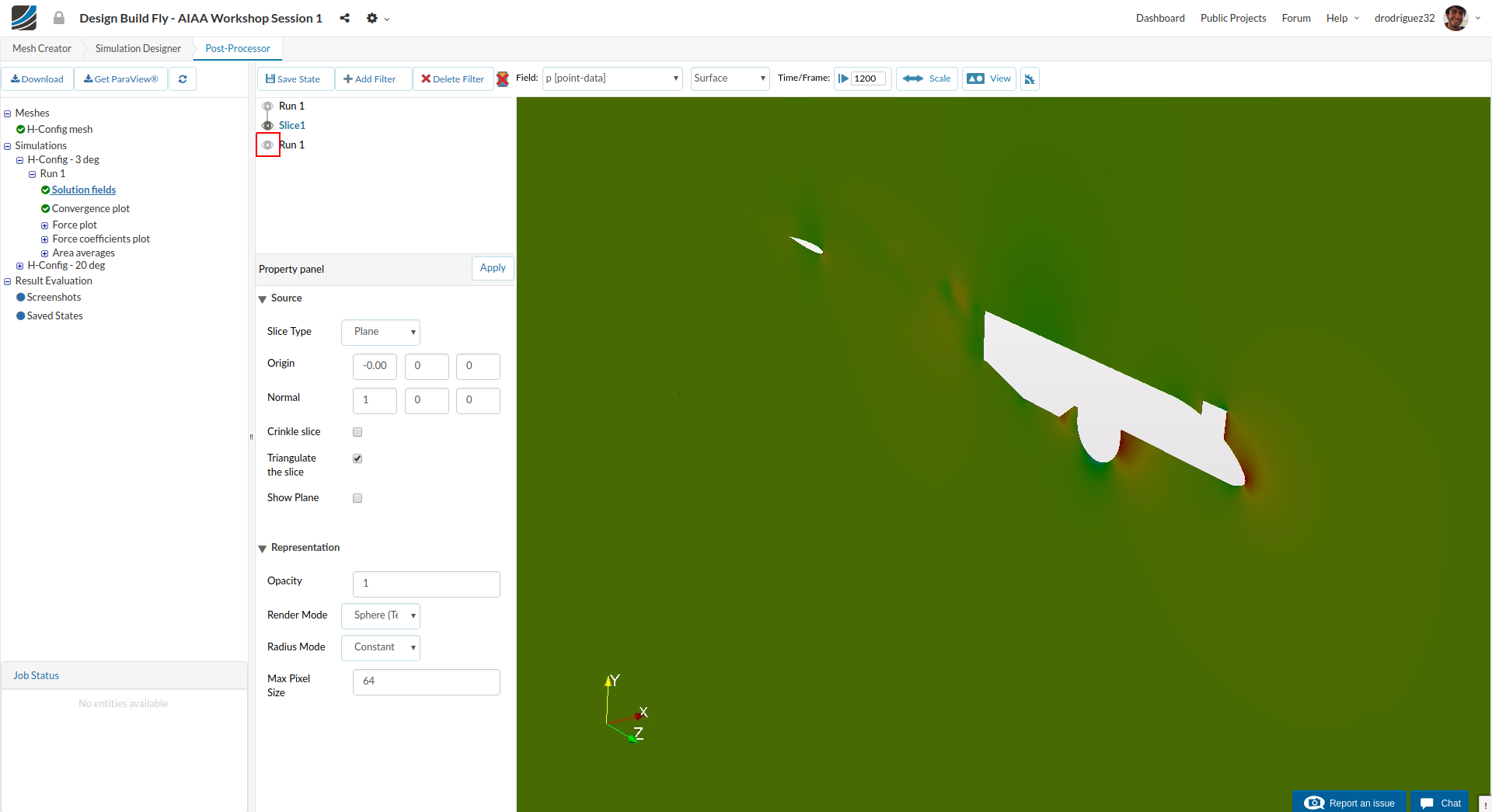
You can hide the airplane to get a better look at the slice.
Velocity
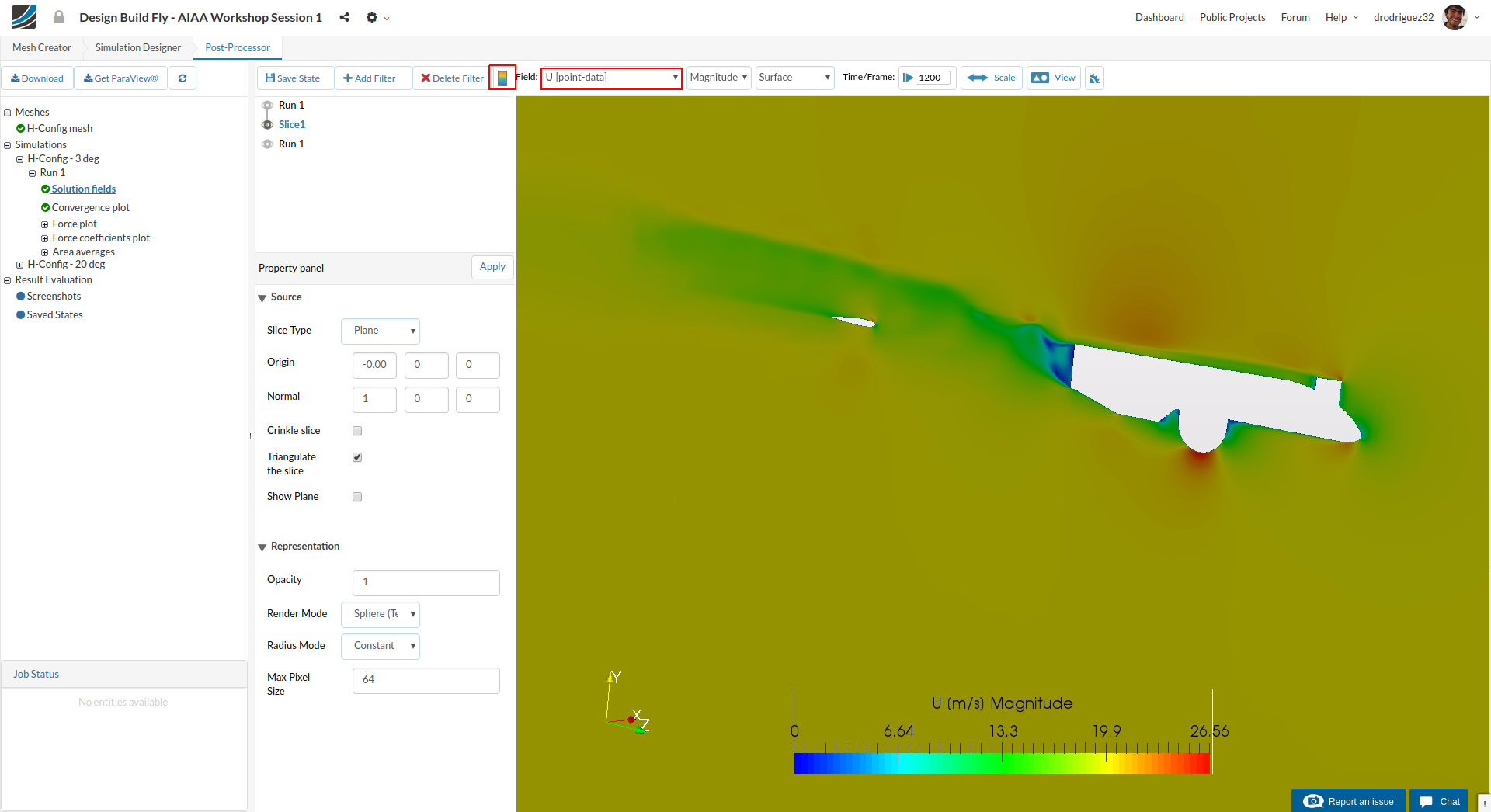
Change the Field to U [point-data] in order to see the velocity field. Zoom the results with the mouse roller and drag from middle mouse button to get a reasonable view. Turn on the color bar and drag it by holding mouse left button to the bottom.
Streamlines
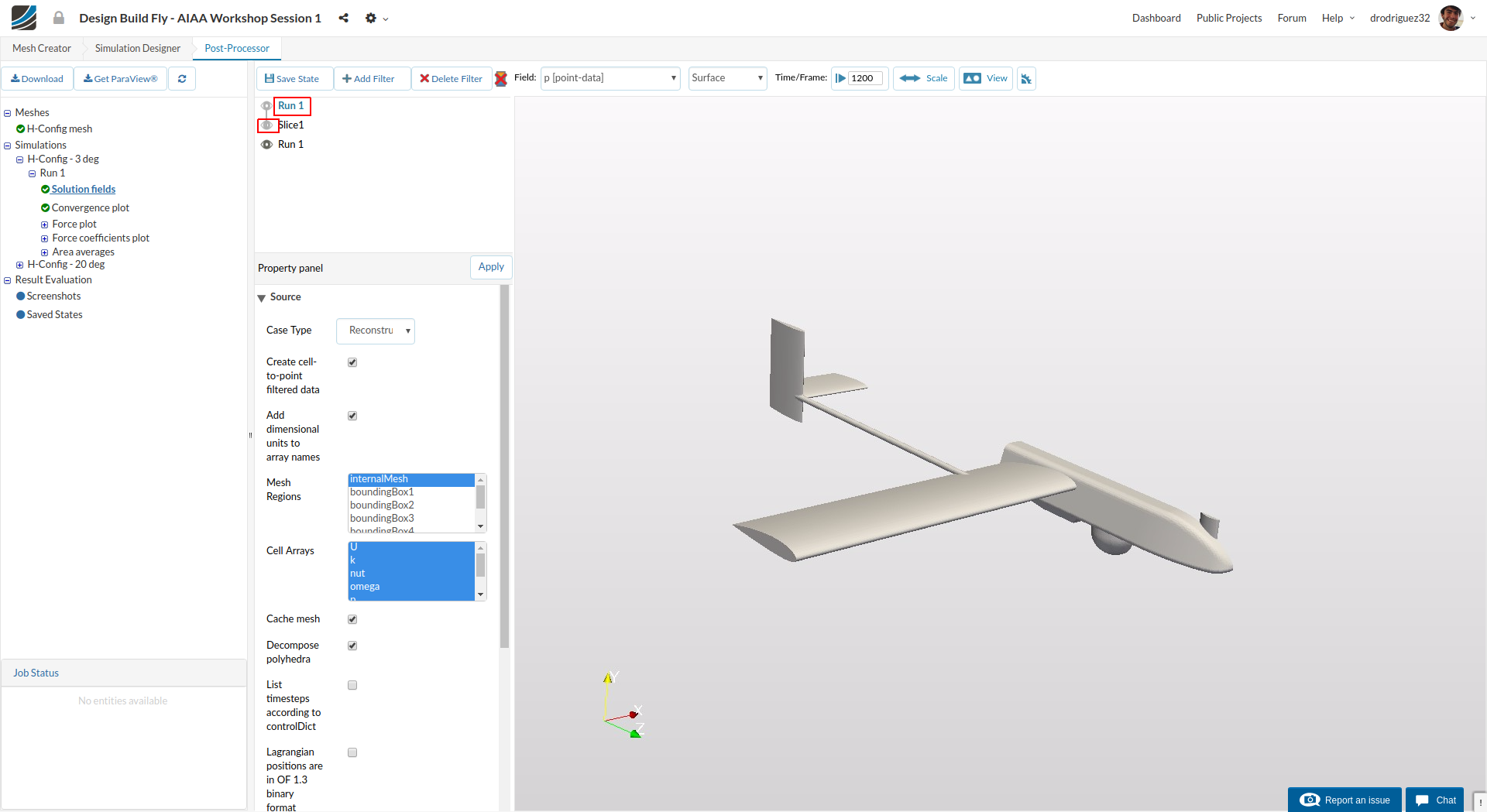
Click on the small eye next to the slice to hide it. And do the same for the result with the surfaces in order to see the plane.
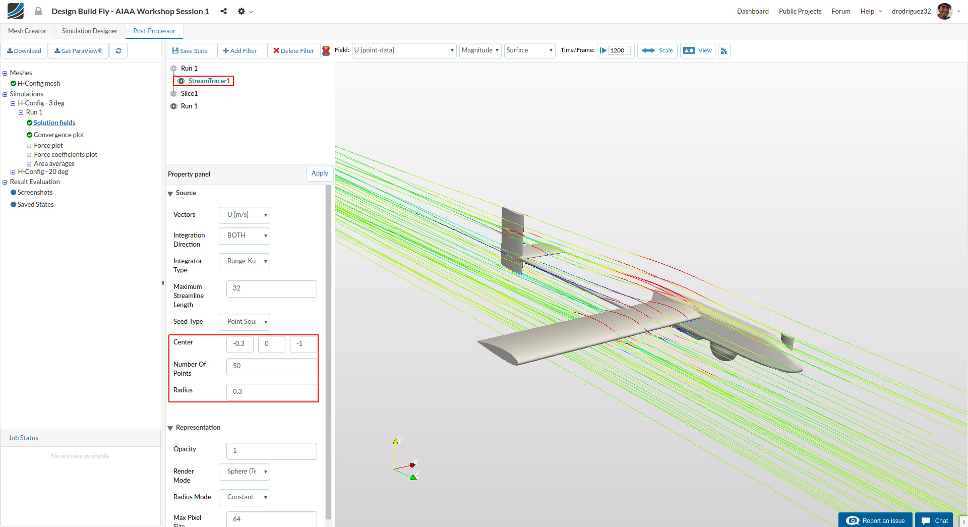
Make sure you click on the first set of results, select Add Filter and then select Stream tracer.
You are free to play around with the Center and Number of Points to get a visualization you like. You can also choose what field you want to visualize, and remember to turn on the color bar. For this case we used:
- Center: (-0.3, 0, -1)
- Number of points: 50
- Radius: 0.3
- Field: U [point-data]
Pressure Distribution on Plane
Hide the Stream Tracer by clicking on the eye to the left of it. And click on the second set of results (the one that has the surfaces)
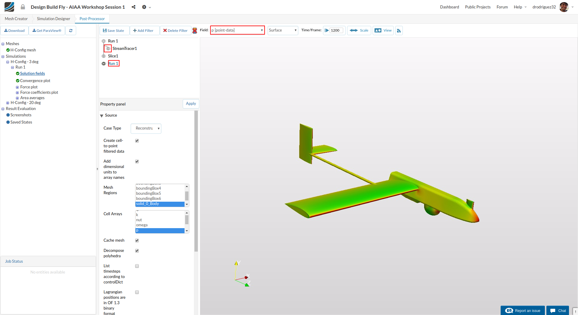
Under Field select p [point-data]. This will show you the pressure distribution on the surface of the plane.
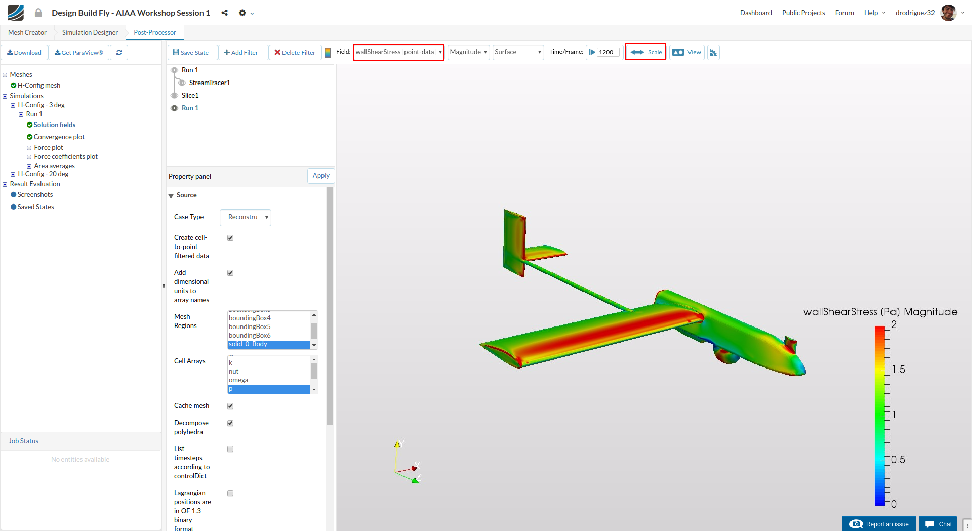
You can also select wallShearStress [point-data] and rescale it from 0 to 2. In this case you can see that there is no sign change so we are getting no flow separation.
Screenshots & Saved States
Under the button View you can generate a screenshot from the viewer instead of having to screenshot your screen - this will get you a higher quality image.
And besides the Add filter button you can also select Save State which will save the filters you applied for later viewing. This means you don’t have to load everything from the start if you want to check your results again.
Lift & Drag
Finally, the most important part of the results is analyzing lift and drag for the wing of the airplane.
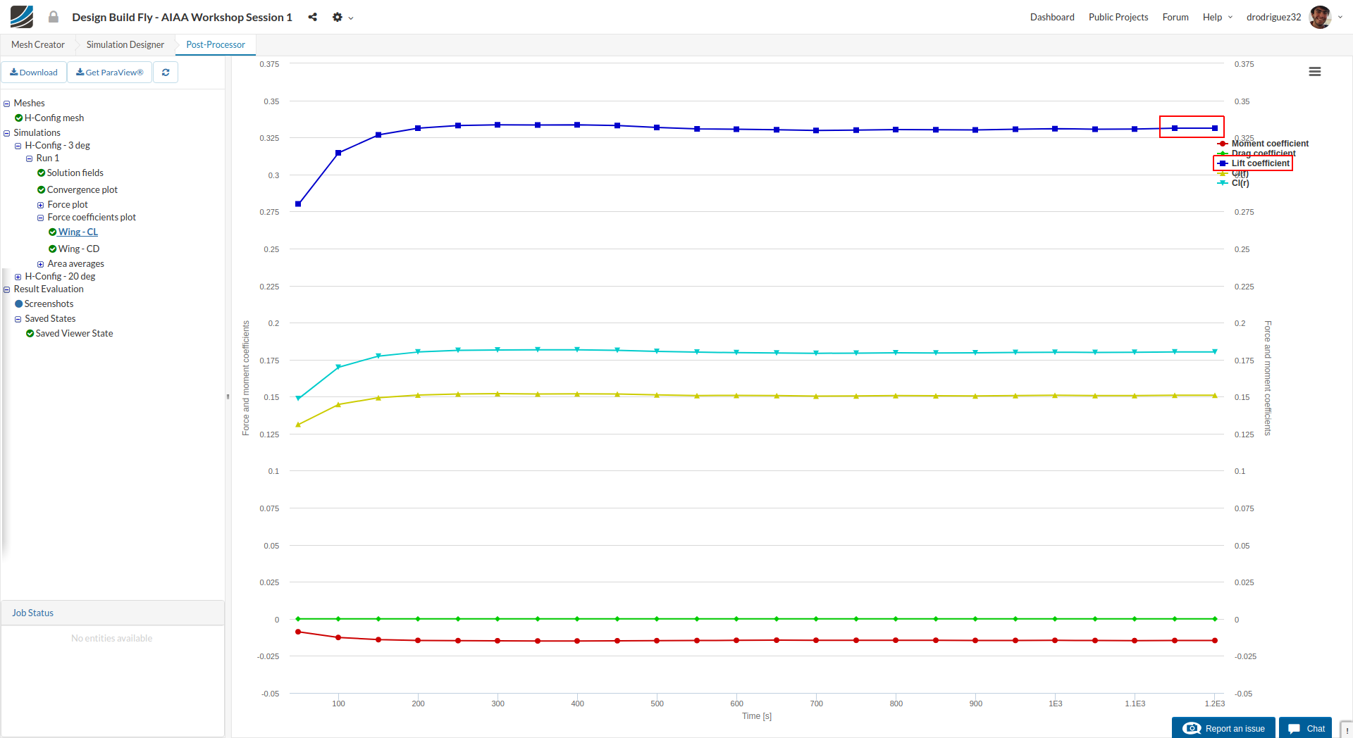
In the Navigator on the left, expand Force coefficients plots and click on Wing - CL. SimScale calculates other coefficients, but in this case we are only interested in Lift Coefficient which for this model airplane is 0.3314
The formula for lift is:
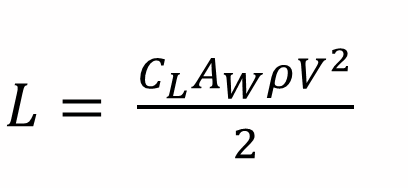
Where:
rho is the density of the air = 1.1965 kg/m3
V is the velocity = 20 m/s
Aw is the reference area = 0.27211108 m2
CL is the Lift Coefficient = 0.3314
By plugging in the numbers we get that each wing produces 21.6 N of lift.
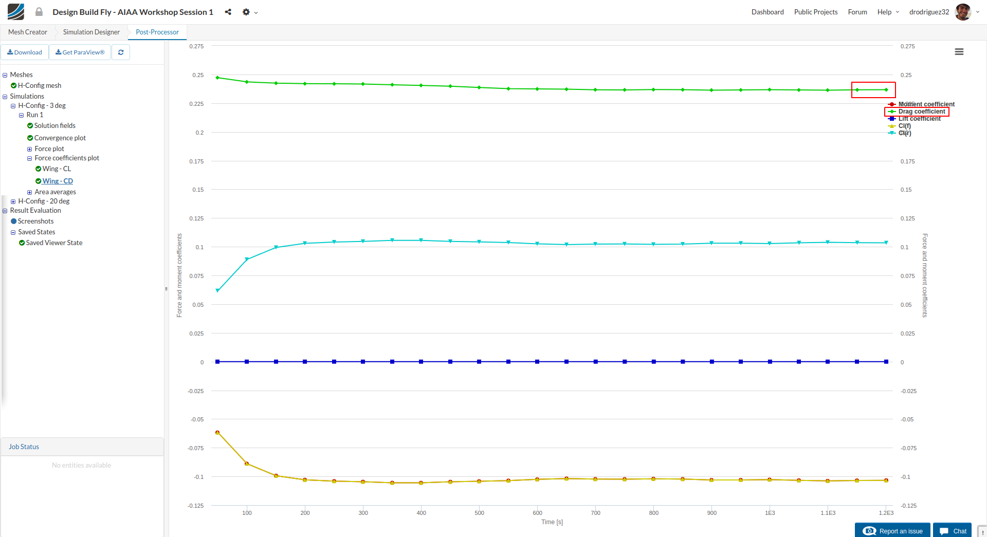
Now click on Wing - CD under Force coefficients plots and this time look at Drag Coefficient which is 0.03305
The formula for drag is:
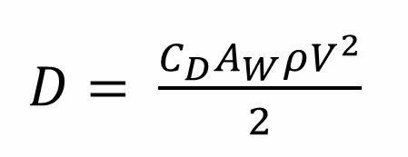
Where:
rho is the density of the air = 1.1965 kg/m3
V is the velocity = 20 m/s
Aw is the reference area = 0.03840402 m2
CD is the Drag Coefficient = 0.03305
By plugging in the numbers we get that each wing produces 2.2 N of drag.

