This post is a continuation of Workshop 2 Session 1- Part I Meshing and it contains the tutorial to setup the simulation for Aircraft wing/blended winglet .
Simulation Setup
We will start off with the Aircraft wing geometry. So navigate to the corresponding Incompressible simulation in the simulation tree. The flow is assumed to be Incompressible due to velocities being less than Mach 0.3. Choosing Steady-State option means that we will simulate the Time-Independent solution.

In the simulation tree, some entries will have a red icon next to them. This means that they have to be completed. Entries ticked in green mean that enough information has been provided (although you can input different values as you deem necessary).
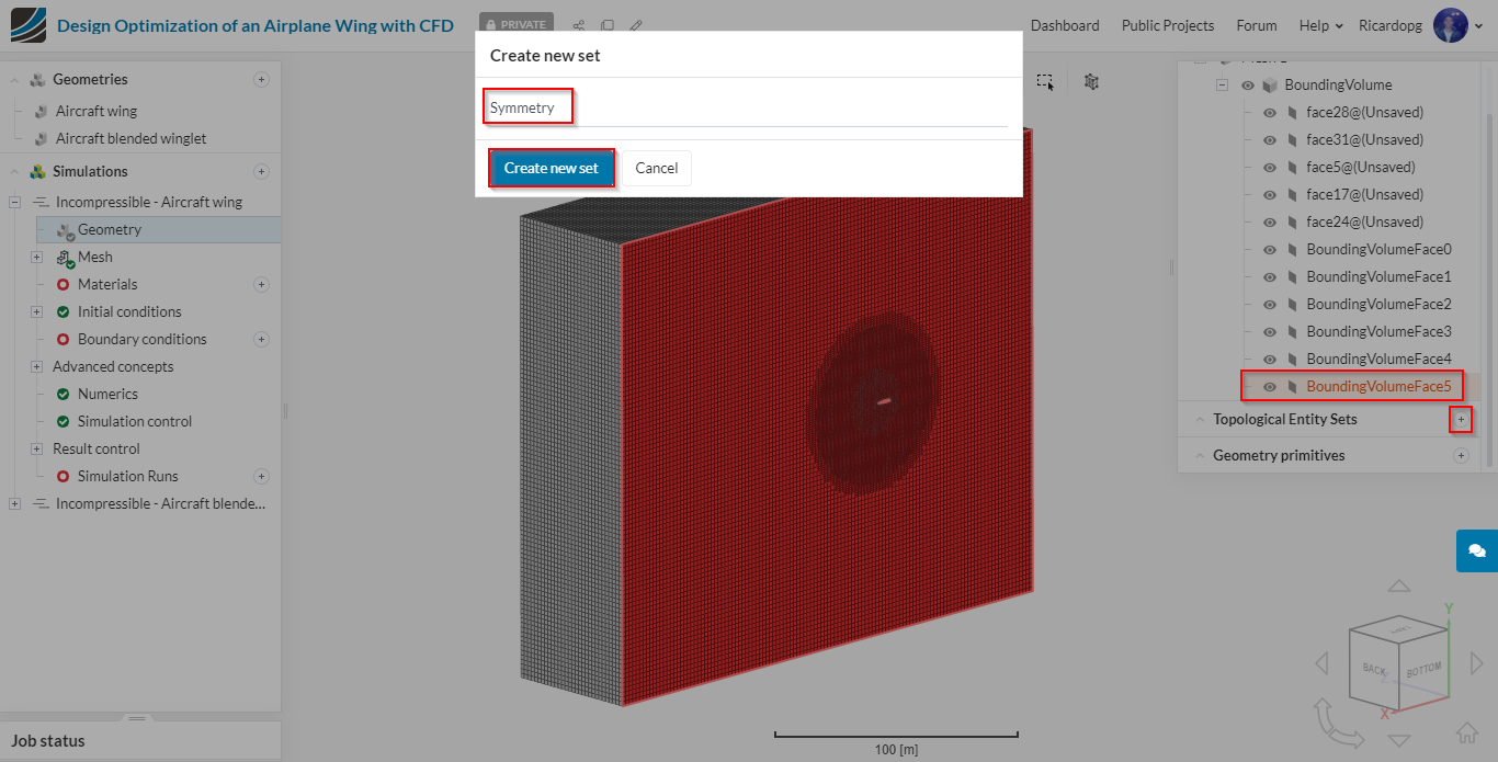
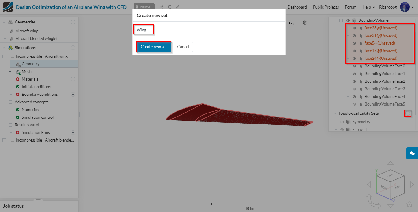
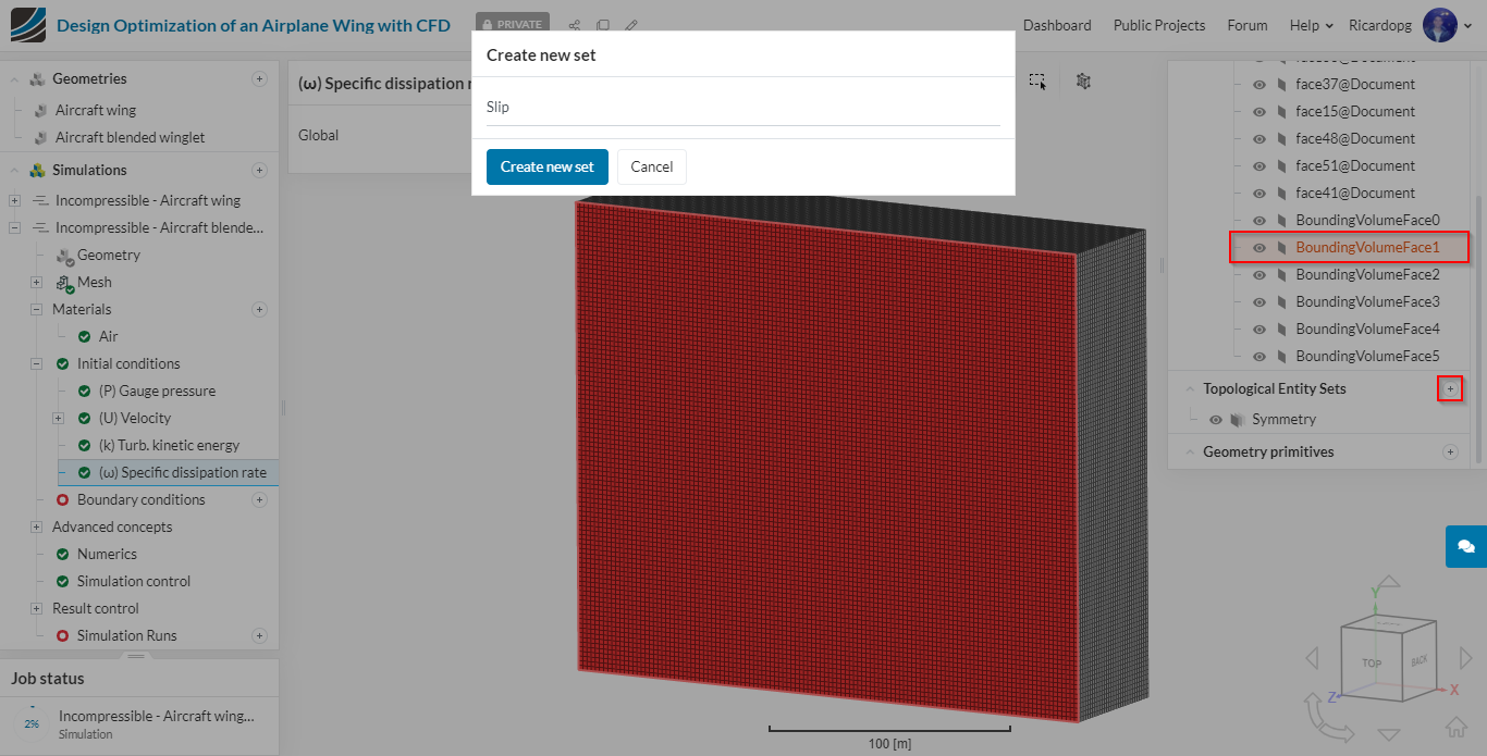
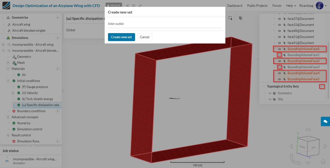
Let’s assign some Topological Entity Sets to make face selection easier throughout the setup. To create Topological Entity Sets, the following steps have to be followed:
- Select the face or faces that will be part of the newly created set;
- On the right-hand side of the screen, next to Topological Entity Sets, click on the + sign;
- Name the new entity set as you deem suitable.
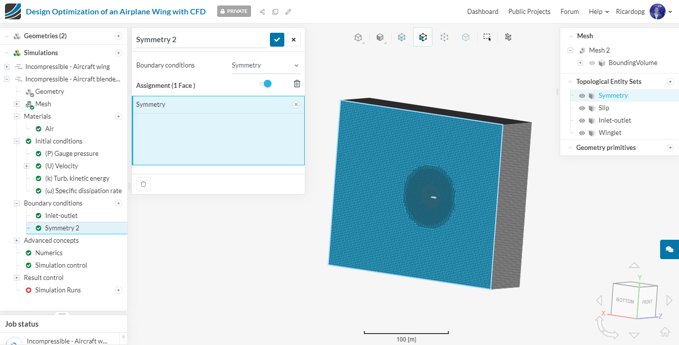
To create a Symmetry entity set, please follow the steps above:
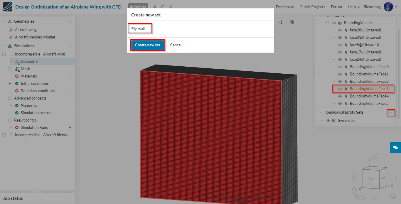
To create a Slip wall entity set, please follow the steps above:
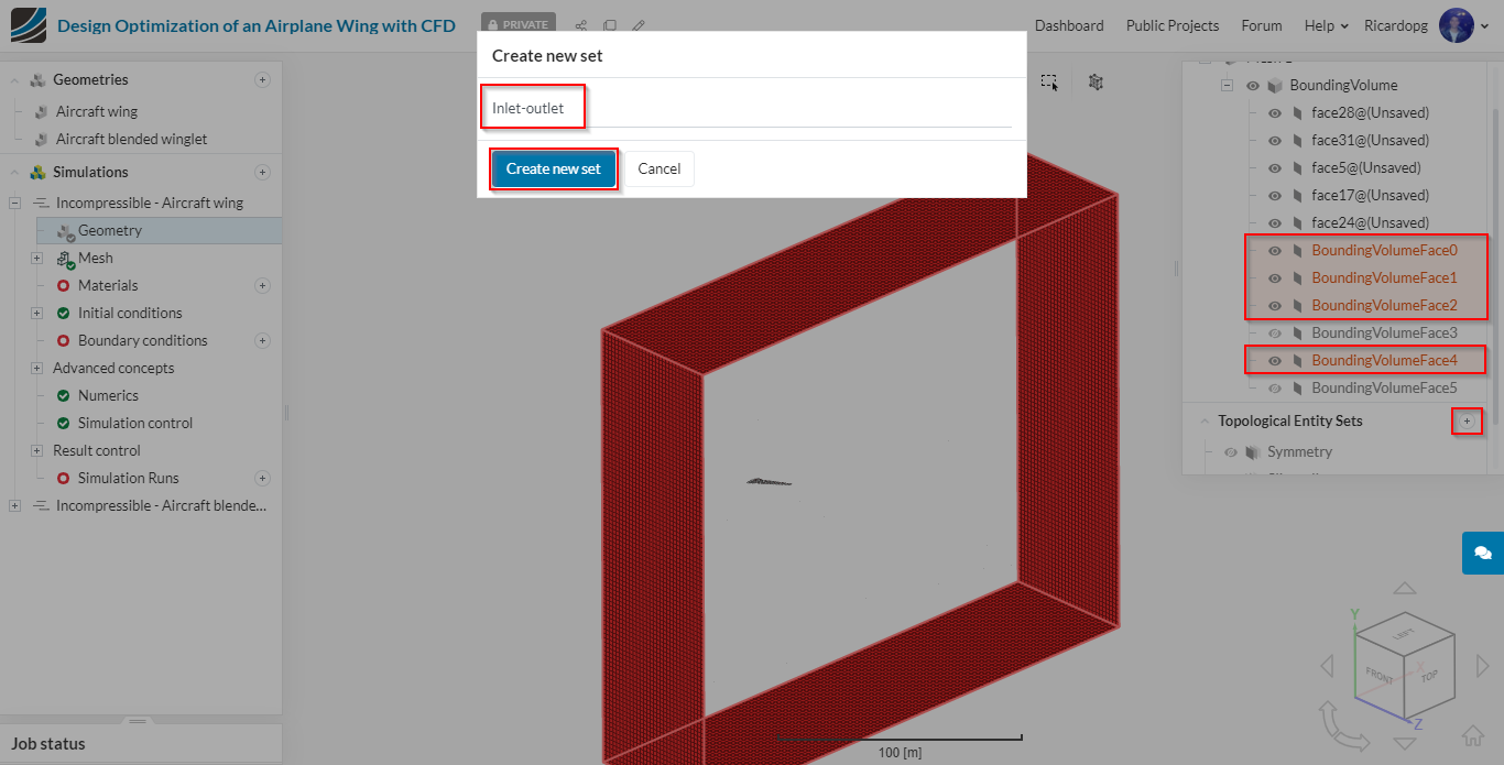
To create an Inlet-outlet entity set, please follow the steps above:
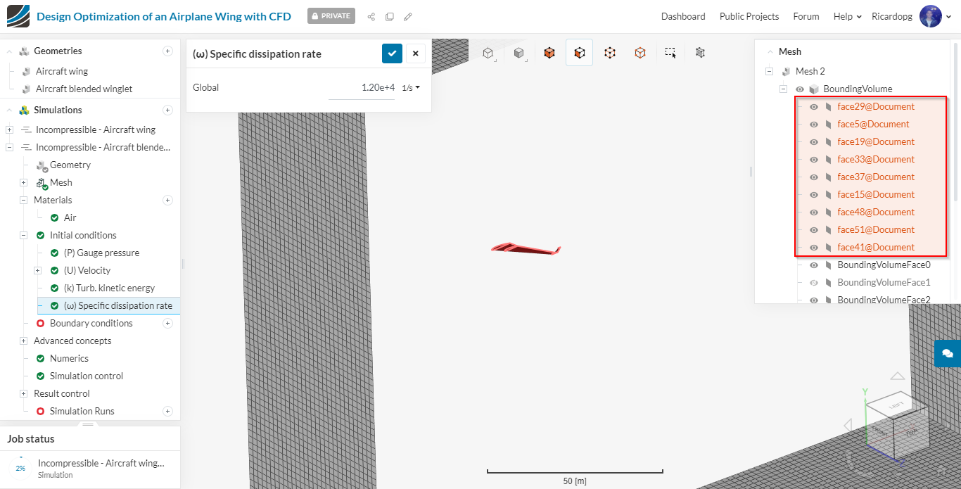
To create a Wing entity set, please follow the steps above:
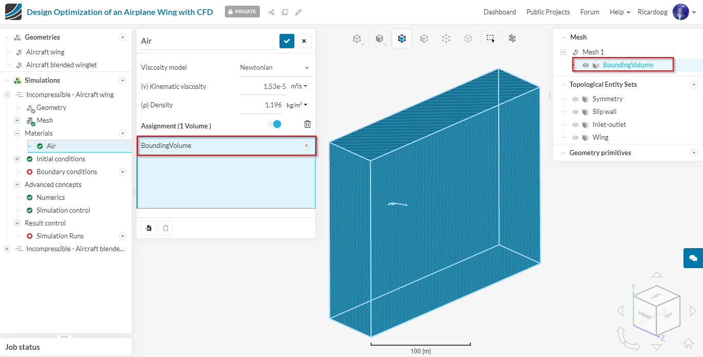
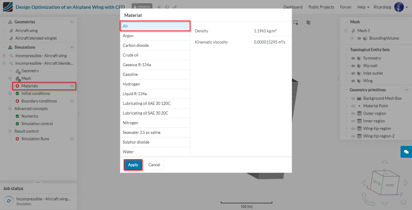
Now, please head over to Materials in the simulation tree. A library of materials will be loaded. Select Air and Apply.
The BoundingVolume is automatically assigned.
Initial Conditions
The Initial conditions are assigned to the whole domain at the start of a simulation. During a simulation, the solver tries to converge the solution fields after taking these initial condition values as a starting point. Therefore, it is important to assign best guesses or analytical solutions as initial conditions when possible.
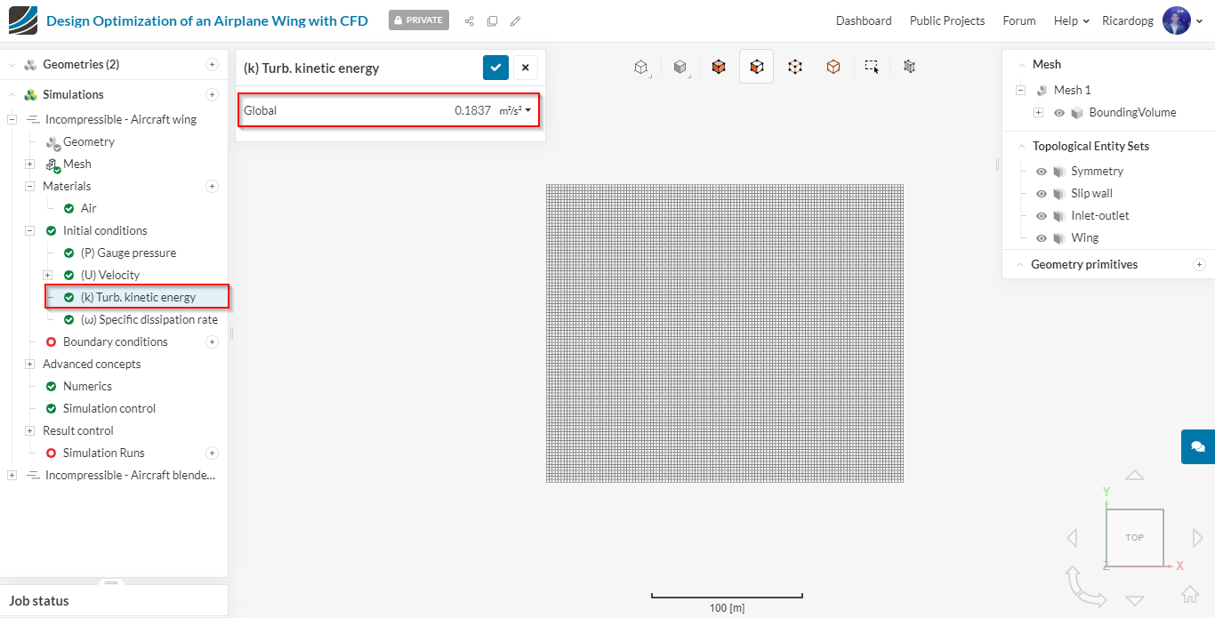
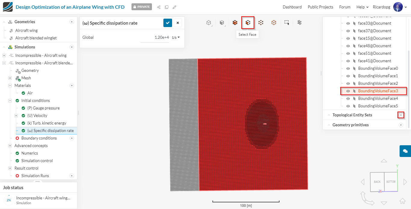
One of the biggest difficulties is estimating (k) Turb. kinetic energy and (ω) Specific dissipation rate. Here you can find some commonly used formulas and also a calculator based on said formulas.
For external flow around cars and even airplanes, it’s common to assume a low turbulence intensity, in the order of 0.5% to 1%. To estimate omega for external flows, we also have to estimate the eddy viscosity ratio:
Eddy Viscosity Ratio ={μt \over μ}
A fair estimate for eddy viscosity ratio in low turbulence is around 1. Therefore, we have the following estimates for k and ω:
k=1.5*(U*I)^2=1.5*(70*0.005)^2=0.18375 {m² \over s²}
ω={k \over ν}*{1 \over {μt \over μ}} =12010 {1 \over s}
Please input these values in the corresponding Initial condition:

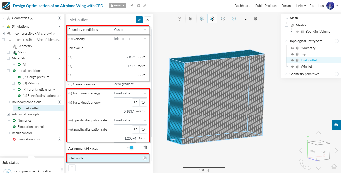
Boundary Conditions
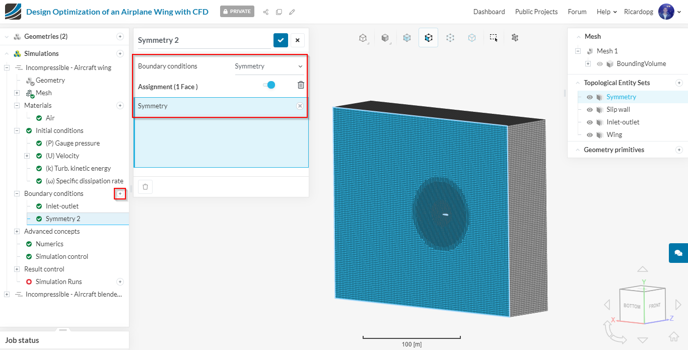
The boundary conditions define the flow variables at the boundary surfaces. To assign a new boundary condition, click on the + sign next to Boundary conditions in the simulation tree.
Inlet-outlet boundary condition:

Symmetry boundary condition:
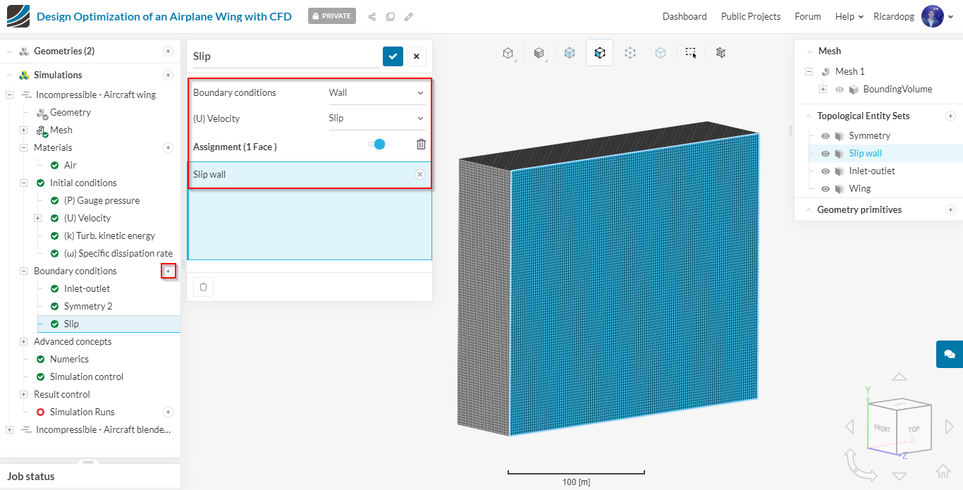
Slip boundary condition:
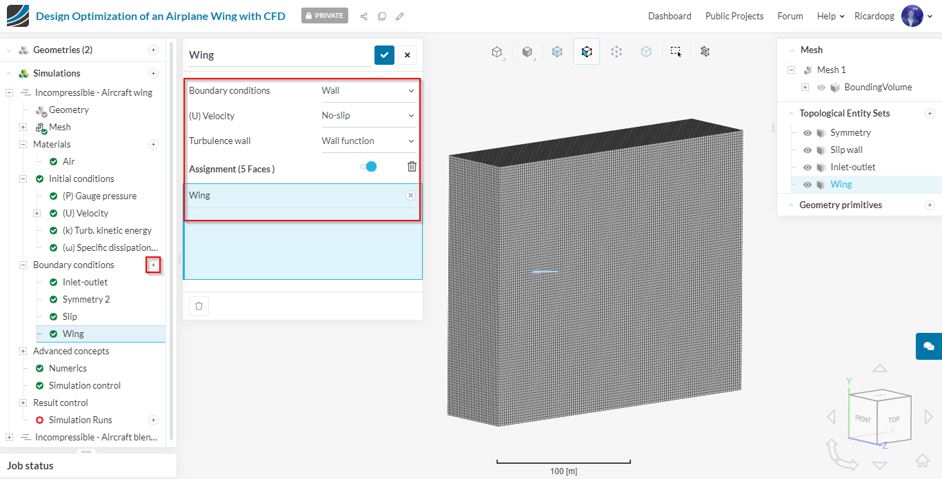
Wing boundary condition:
Numerics
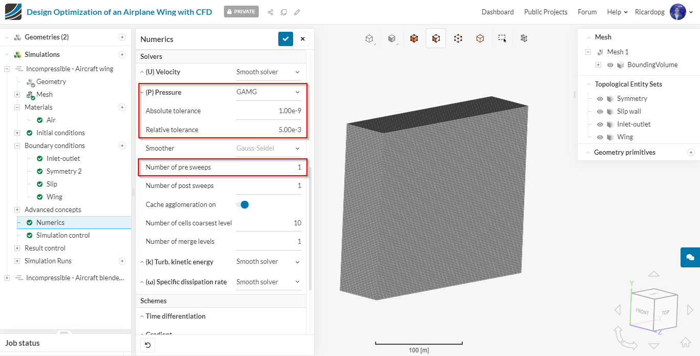
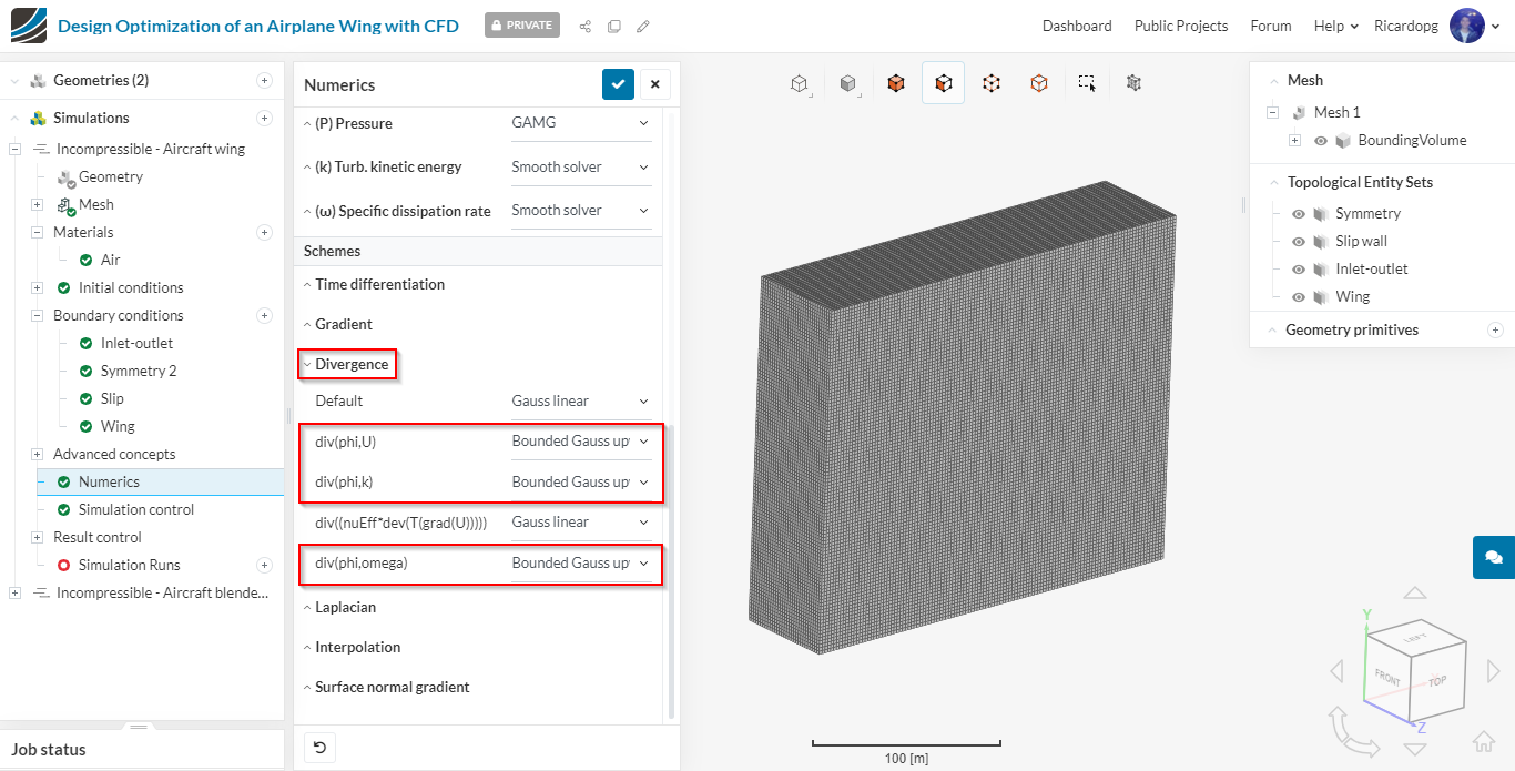
Please select Numerics in the simulation tree. In the numerics panel that opens up, scroll down to find Solvers. Click on ( P ) Pressure to enlarge. Please adjust the settings as shown:
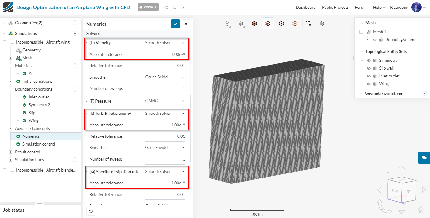
Now enlarge the other 3 solvers (U, k and ω) and set the Absolute tolerance for each one of them to 1e-9:
Scrolling down a little further, you will see Schemes. Enlarge the Divergence schemes and change div(phi,U), div(phi,k) and div(phi,omega) to Bounded Gauss Upwind.
For the Laplacian schemes, please change all entries to Gauss linear corrected:

Simulation control
Just below Numerics, you can find the Simulation control settings. Please increase Maximum runtime to 30000 seconds. Also enable Potential foam initialization, which initializes the velocity field.
The number of processors that will be used for the simulation is automatically optimized, based on the job size.

Result control
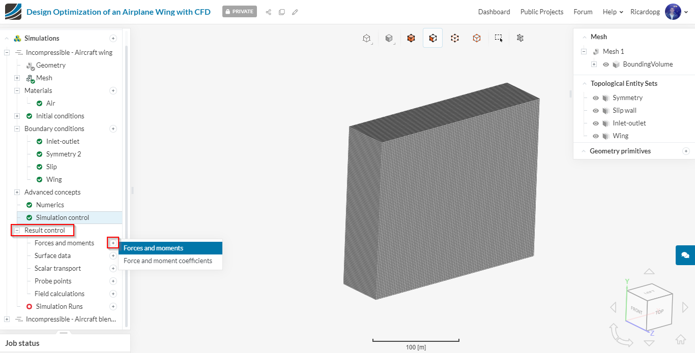
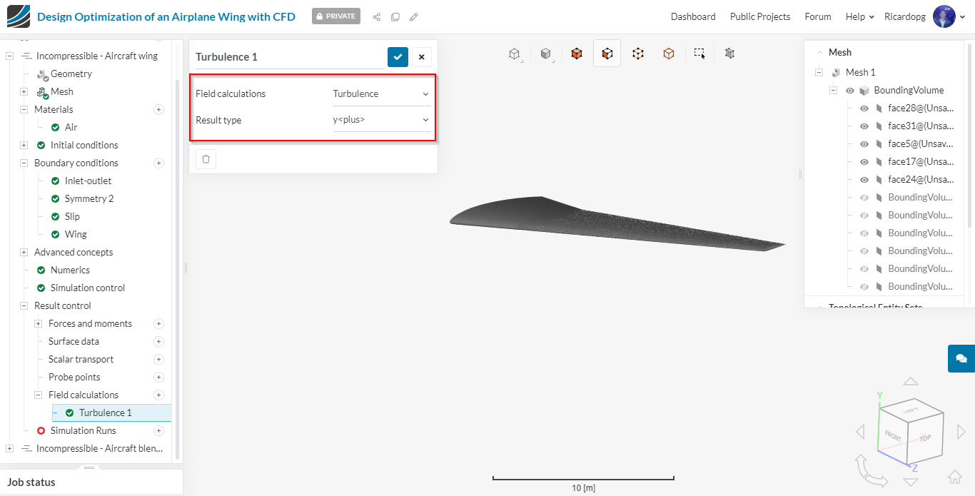
It’s important to set result controls in order to assess convergence and also to generate important information for the post-processing phase. We will add a Forces and moments control, aswell as a Turbulence control for yPlus.
To add a Forces and moments, kindly follow these steps:
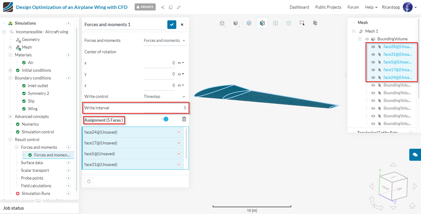
Change the Write interval to 5 iterations in order to save some computing time. Select all the wing faces and save:
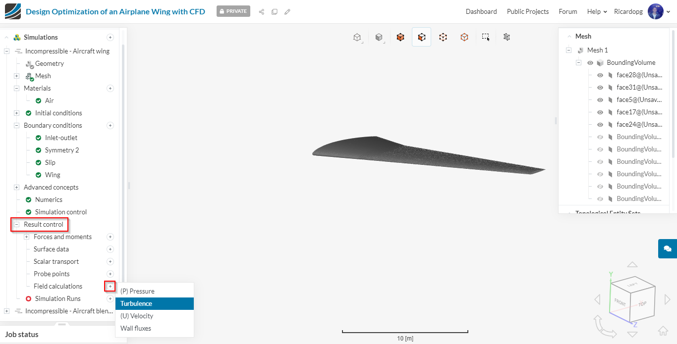
The Turbulence result control can be found under Field calculations
Now we are ready to start our Simulation Run!

Note that in SimScale you can run multiple simulations in parallel. Hence you can start setting up the next case.
Aircraft blended winglet
Now in the simulation tree, expand the second Incompressible simulation, which is linked to the Aircraft blended winglet geometry.
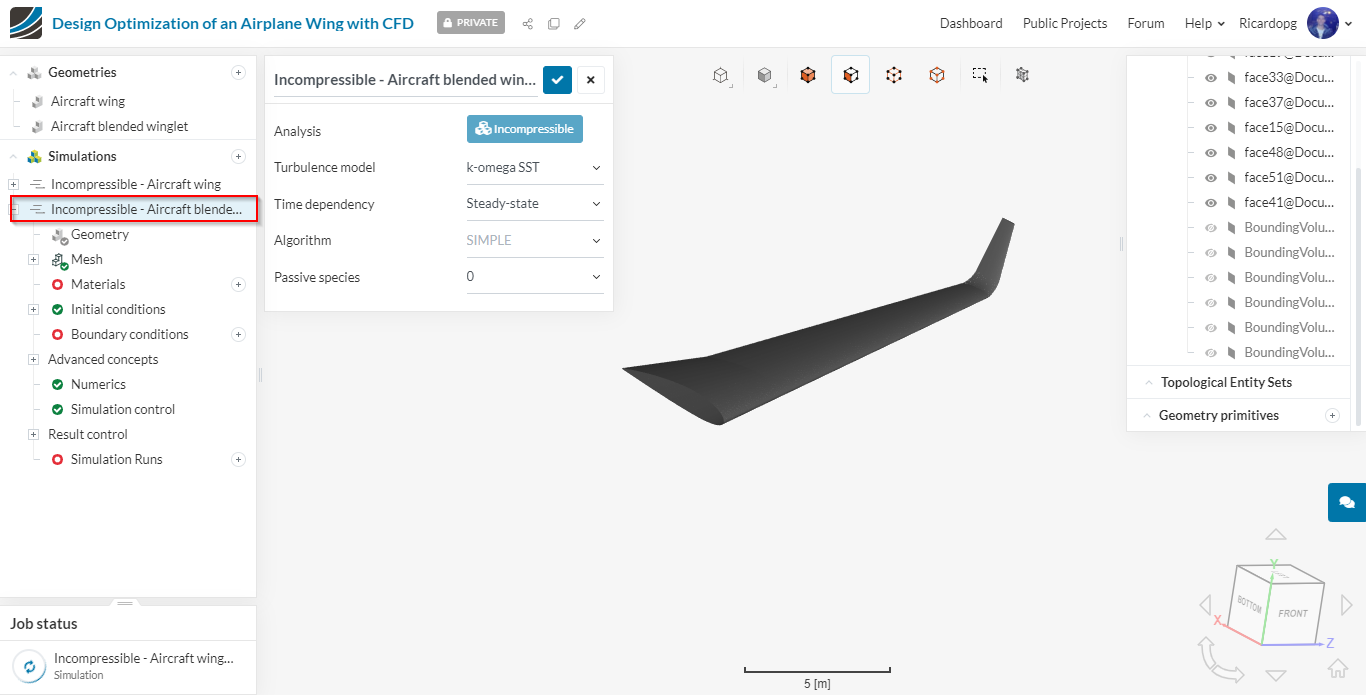
The setup is very similar to the previous geometry, only making some adaptations, remembering that we have a winglet.
Let’s assign air to the BoundingVolume by clicking on Materials:
For Initial conditions, we are going to use the same previously calculated values for (k) Turb. kinetic energy and (ω) Specific dissipation rate:
k=0.18375 {m² \over s²}

ω=12010 {1 \over s}

Now let’s create Topological Entity Sets for the winglet geometry. They will be similar to the entity sets created for the previous geometry. One more time, the steps to create a topological entity set are:
- Select the face or faces that will be part of the newly created set;
- On the right-hand side of the screen, next to Topological Entity Sets, click on the + sign;
- Name the new entity set as you deem suitable.
To create a Symmetry entity set, please follow the steps above:
To create a Slip wall entity set, please follow the steps above:
To create an Inlet-outlet entity set, please follow the steps above:
To create a Winglet entity set, please follow the steps above:
Now we can proceed to creating boundary conditions:
Inlet-outlet boundary condition:
Symmetry boundary condition:
Slip boundary condition:

Winglet boundary condition:

Numerics, Simulation control and Result control are the same as those from the previous simulation. After all of these have been setup, please create a Simulation Run
Post-processing
The simulations take about 90 to 150 minutes to finish running.
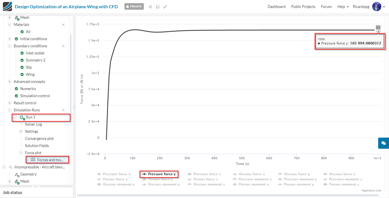
After they are completed, we can inspect the results. First, let’s compare forces in the y direction (lift):
The first geometry (wing without winglets) generates about 166 kN of lift.
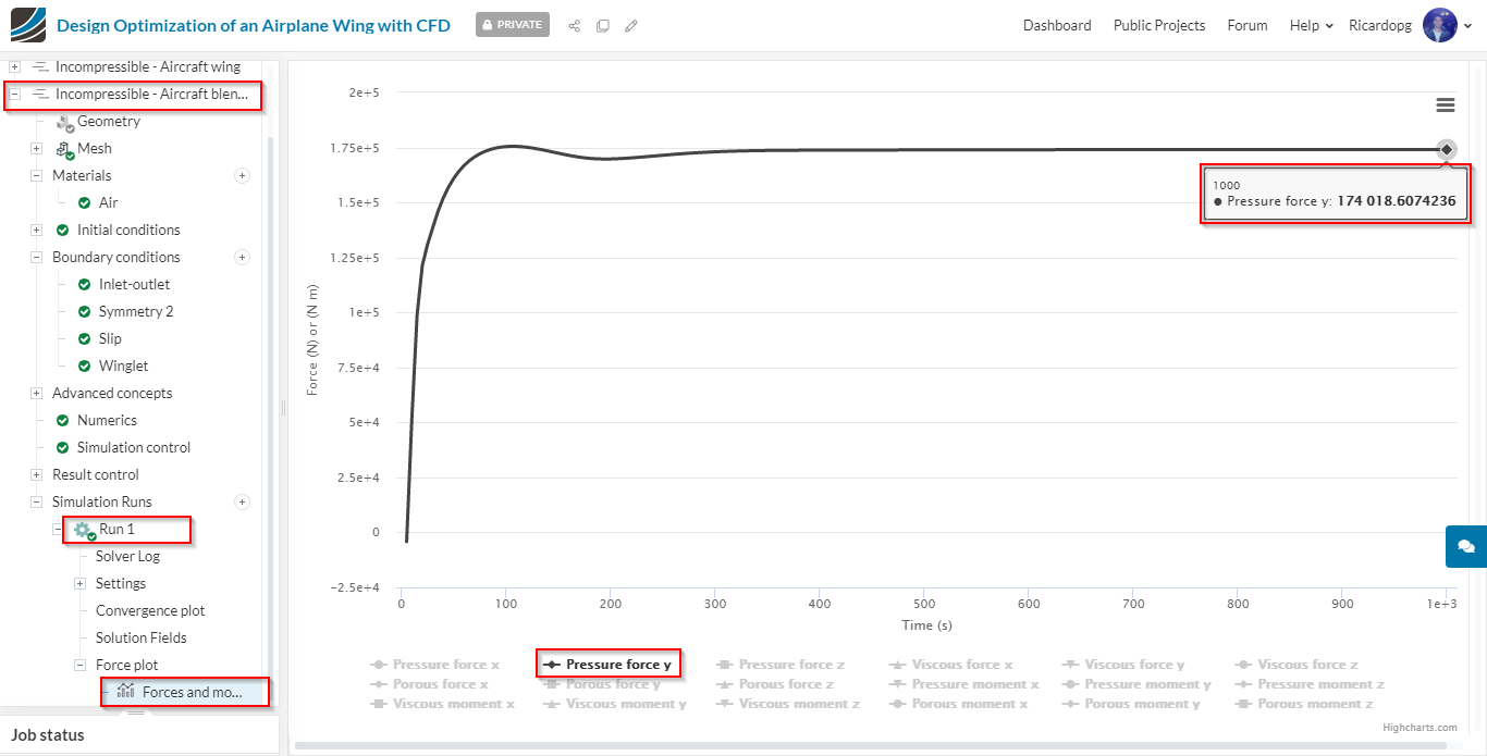
In comparison, the geometry with winglets generates 174 kN of lift. That’s quite a difference.
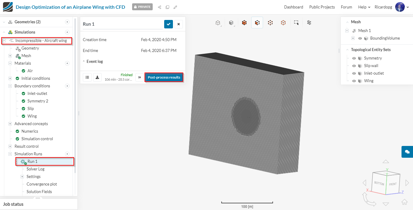
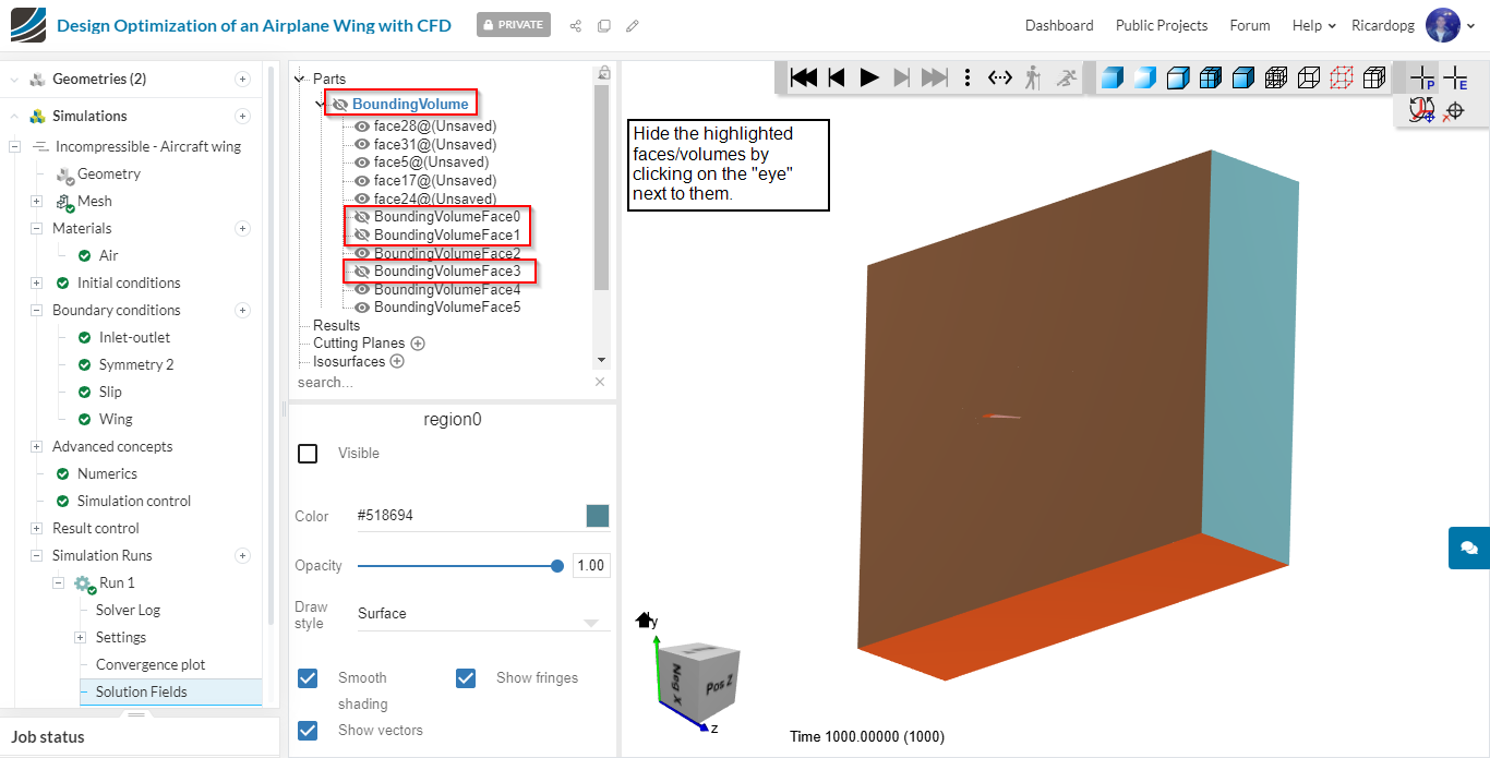
Now, for the winglet-less geometry, let’s head over to the post-processing environment:
Please follow the steps shown below to get pressure contours on the wing and symmetry plane:
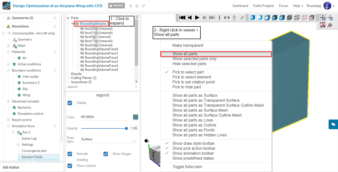
.
Now click on Results and select the desired parameter. Here are screenshots for Pressure contours
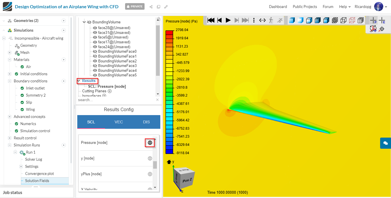
This method is also useful to evaluate yPlus.
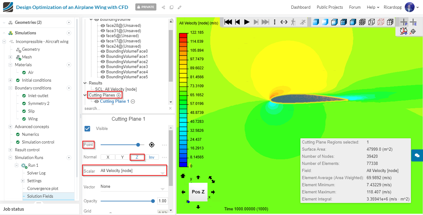
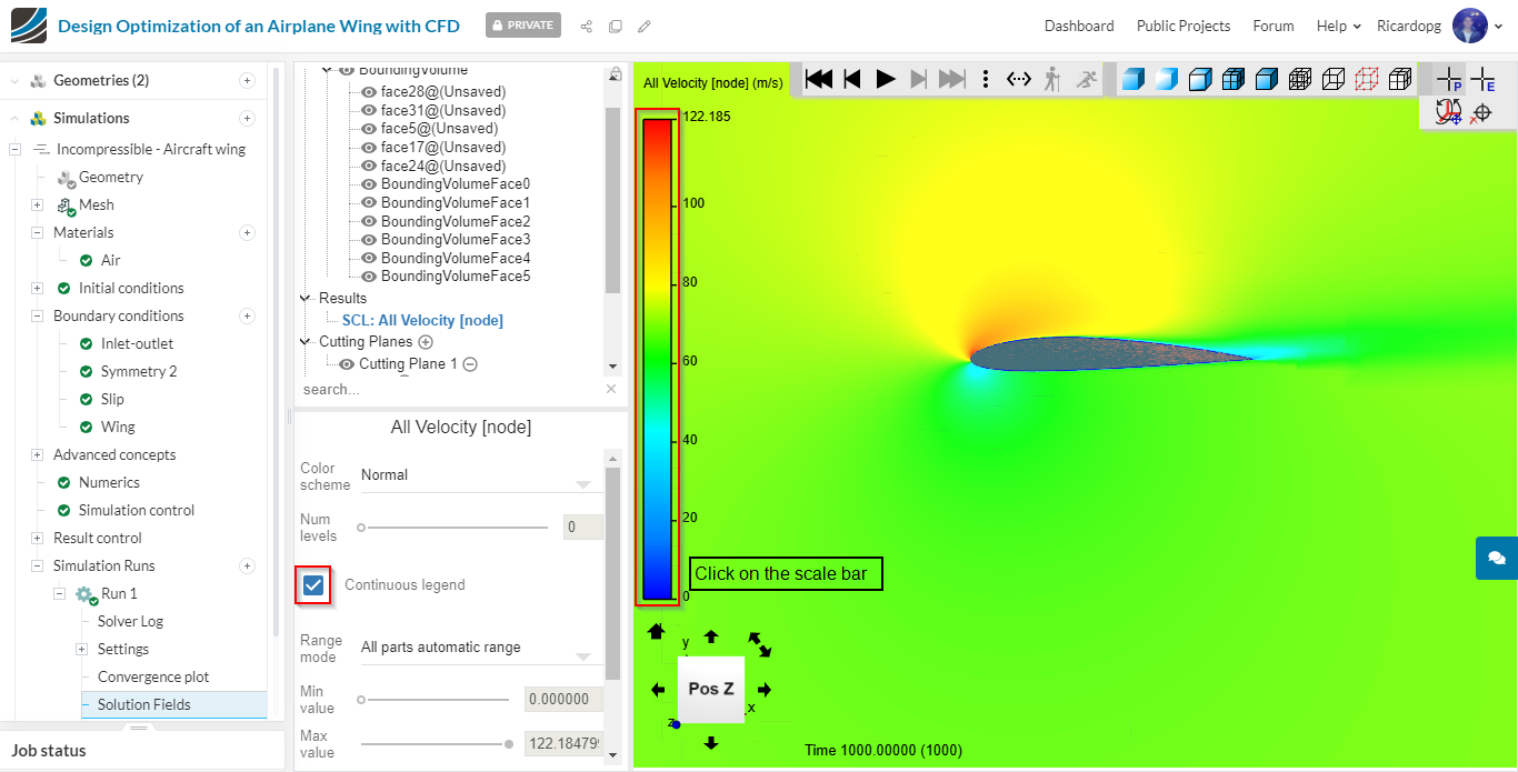
Let’s now create a Cutting plane to see Velocity contours.
First, click on Cutting planes. Make sure that the Z direction is normal to the plane by clicking on Z. Then, next to Point there is a bar that controls the cutting plane placement. Slide it to right side until the wing is visible in the cutting plane.
You can select what parameter will be evaluated in the drop down arrow next to Scalar.
It’s also possible to change scale settings. To do that, please click on the scale, then enable Continous legend. This way the velocity plot has a very smooth visual.
Stream lines
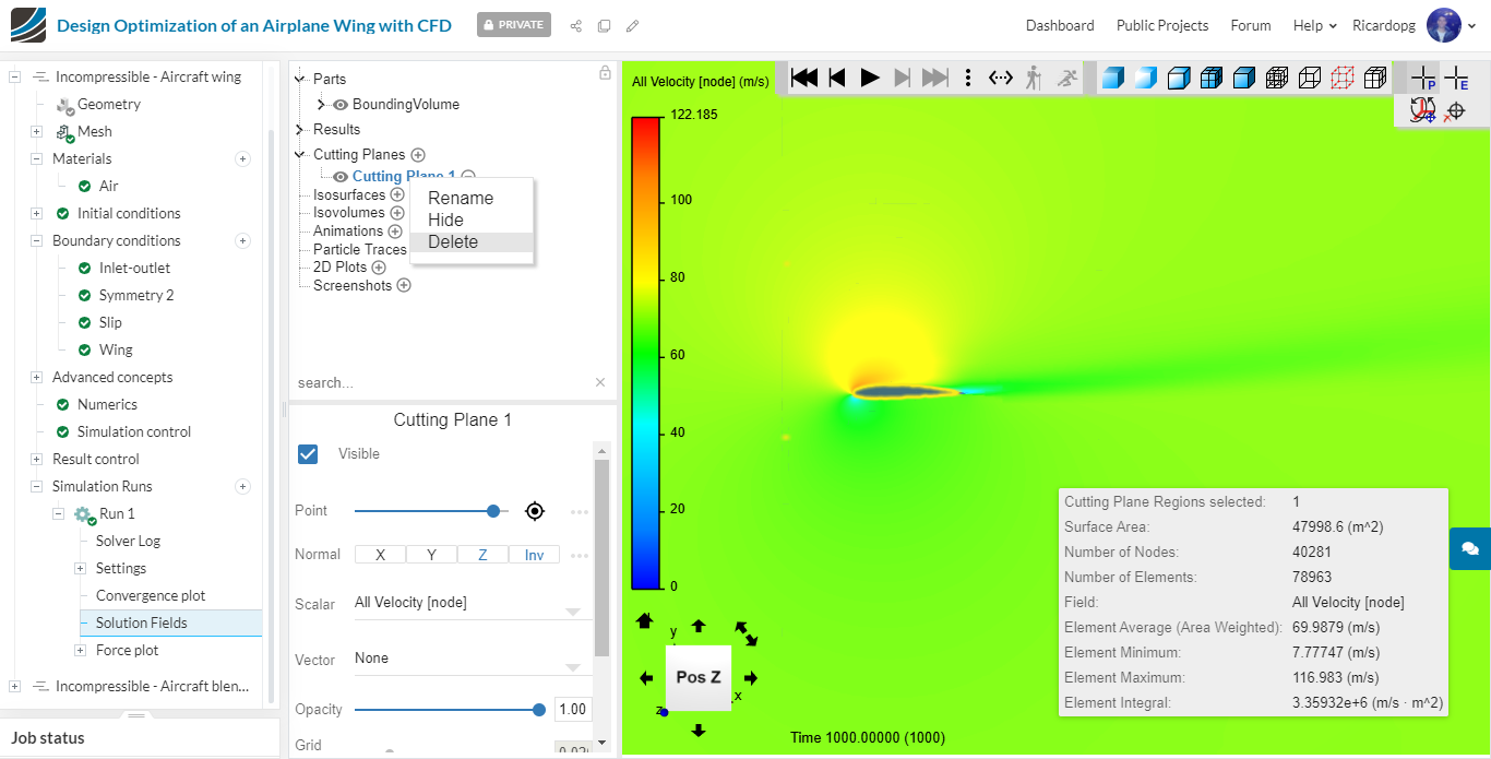
Now please delete the cutting plane by right clicking on it and clicking on Delete.
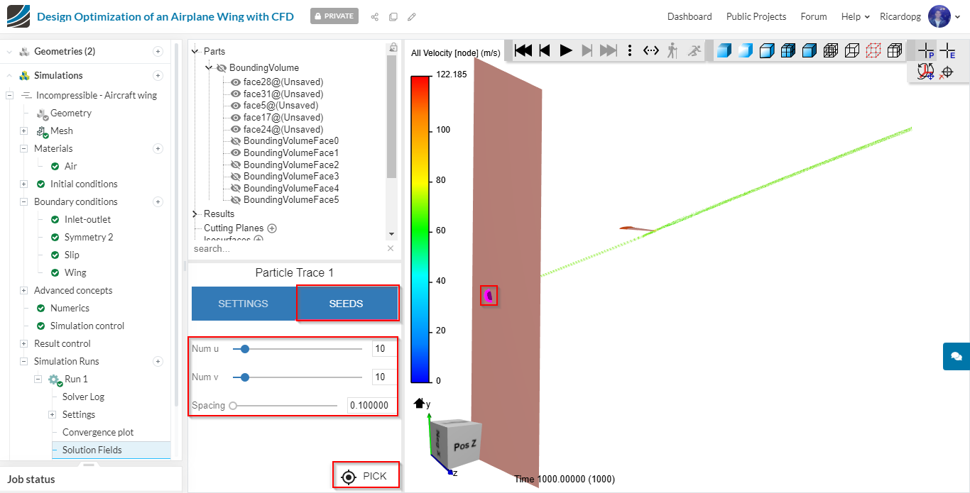
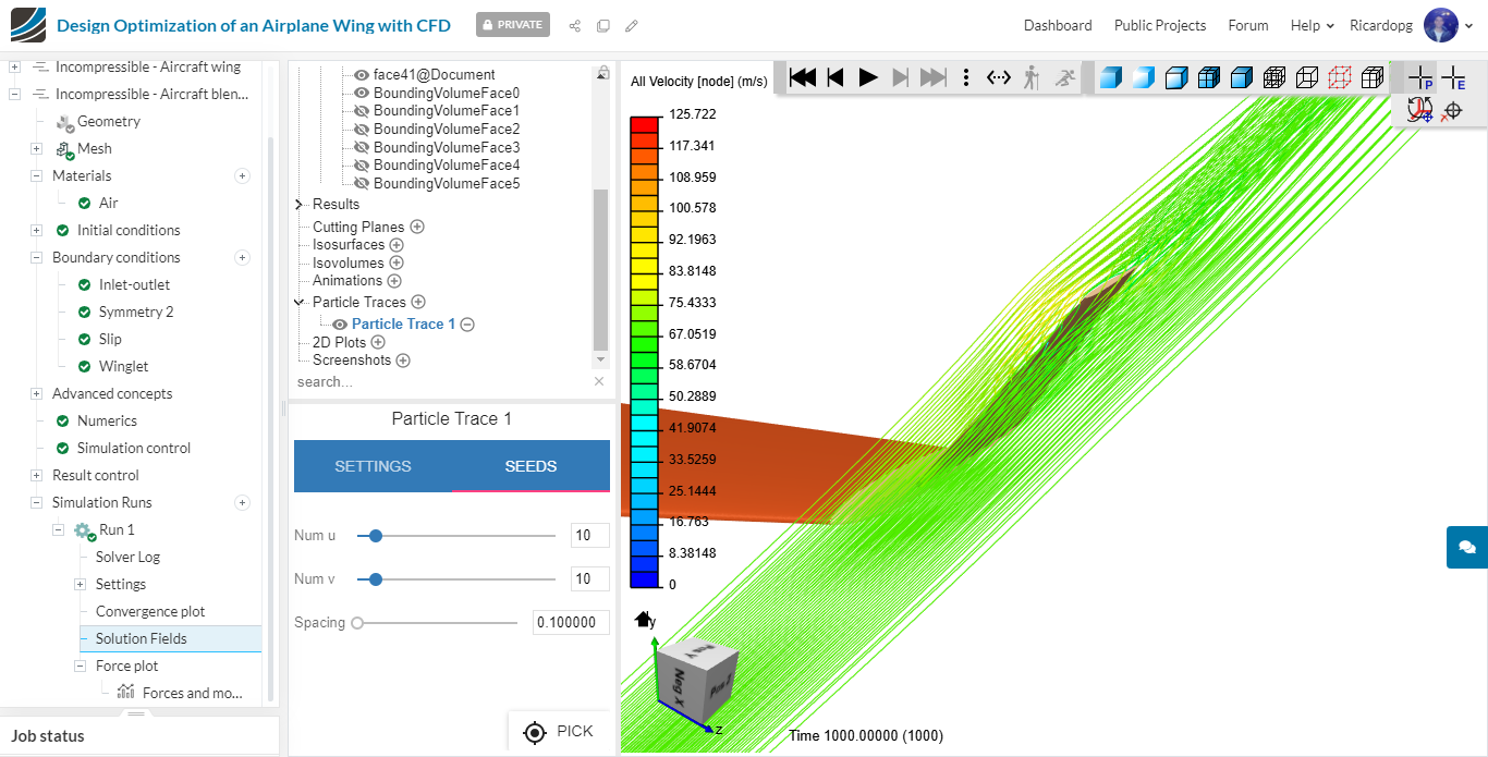
A little further down from Cutting Planes you will find Particle Traces. This function server the purpose of generating flow lines. It is highly customizable. The user can adjust face opacity, shape, radius, number and spacing of flow lines, By clicking on SEEDS and then PICK, the user can select a face from where the traces will be generated.
We can see, for instance, the flow lines around the tip of the wing:
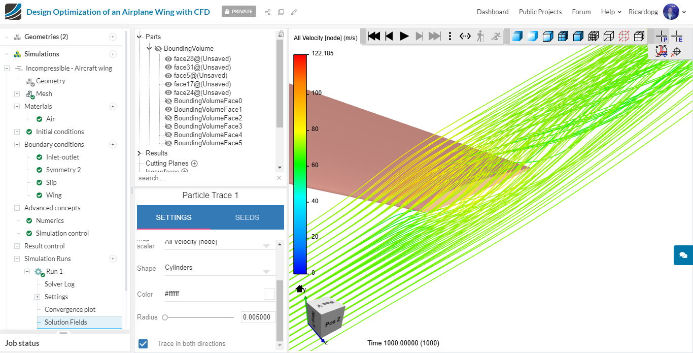
And we can also compare these lines to the geometry with winglets:
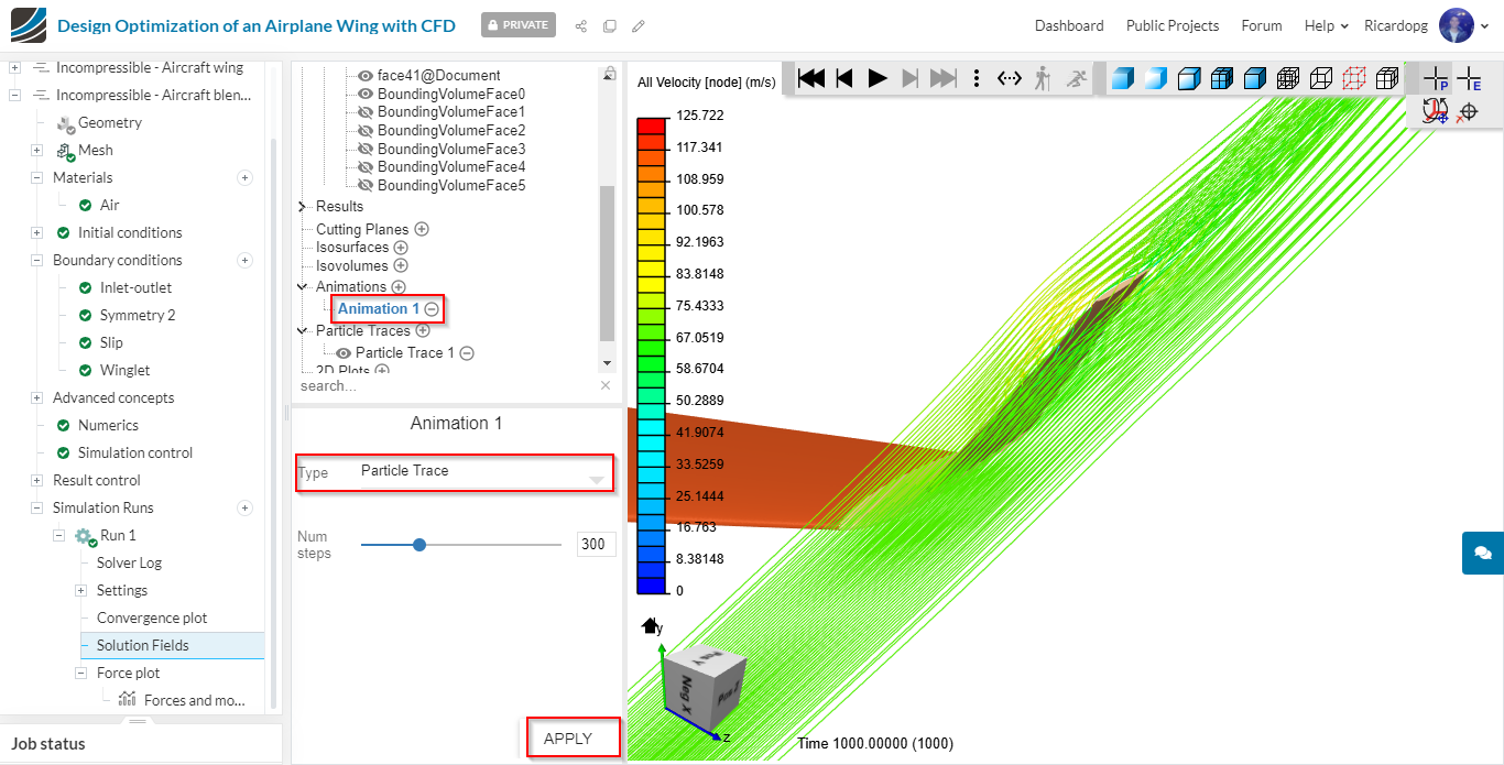
It’s also possible to make an Animation using the flow traces, by clicking on Animations, changing the type to Particle Trace, selecting the total number of steps and hitting APPLY.