NOTE: This tutorial was updated on 08/2016 to match the updated version of the platform
If you would like to watch the first session of the F1 Workshop again or in the case you missed it, you can access the full recording below.

Exercise
Here you have to set up a fully fledged flow simulation of the aerodynamics of a front wing. This simulation will later on enable you to calculate drag and lift forces as well as identify flow separations.
Your task is to investigate the behaviour of drag and lift for a airflow velocity of 40m/s, 50m/s, 60m/s 70m/s and 80m/s
Let’s take a look at the physics of the front wing before we start to set up our simulations:
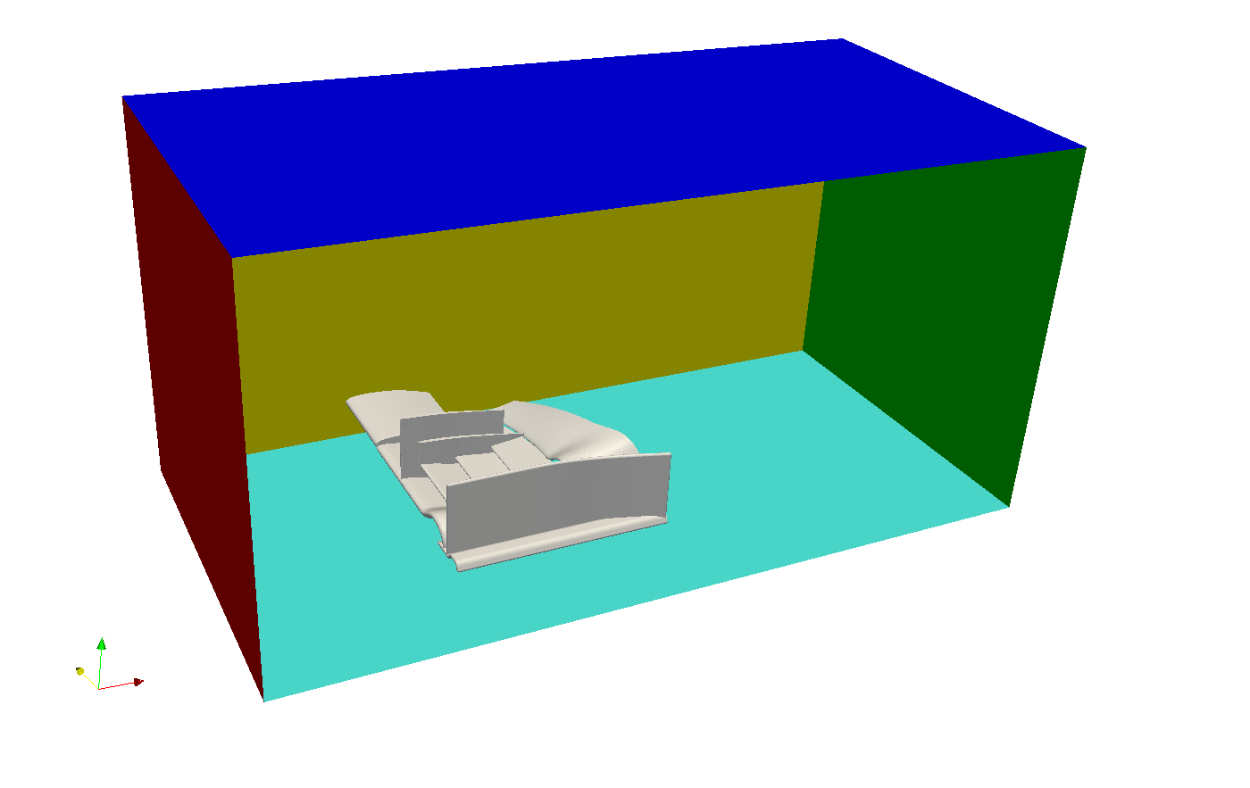
As a first simplification we can exploit the symmetry of the front wing. It is therefore practical to simulate only one half of the wing to reduce the computational effort by defining the inner surrounding wall (yellow) as a symmetry plane.
The body of the wing is a physical wall (grey), which means that it involves friction. This faces should be considered as non-slip walls.
The outer and upper surrounding walls (blue) are necessary to limit the domain we want to simulate, since we are not able to simulate an infinitely large domain. Nevertheless they do not exist in reality and should therefore not interact with the flow. A good approximation here is to assume this wall as frictionless or so-called slip walls.
There is no relative motion between the air and the floor since the car is driving thourgh our domain. We will therefore apply a wall velocity on the lower sorrounding wall (cyan)
The bounding face on the left-hand side (red) will be defined as a inlet with a constant flow velocity profile.
The bounding face on the right-hand side (green) will be defined as a outlet with a constant pressure.
Step-by-Step instruction:
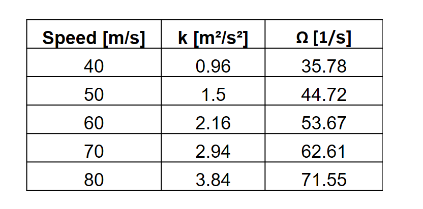
Note: These instructions refer to the simulation setup for a airflow velocity of 60m/s. For the other velocities you have to adapt also the initial values for k and omega which you can find in the table below:
Meshing:
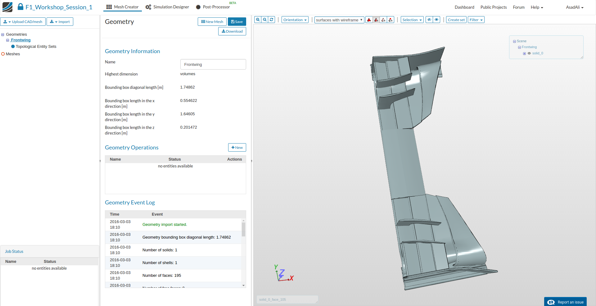
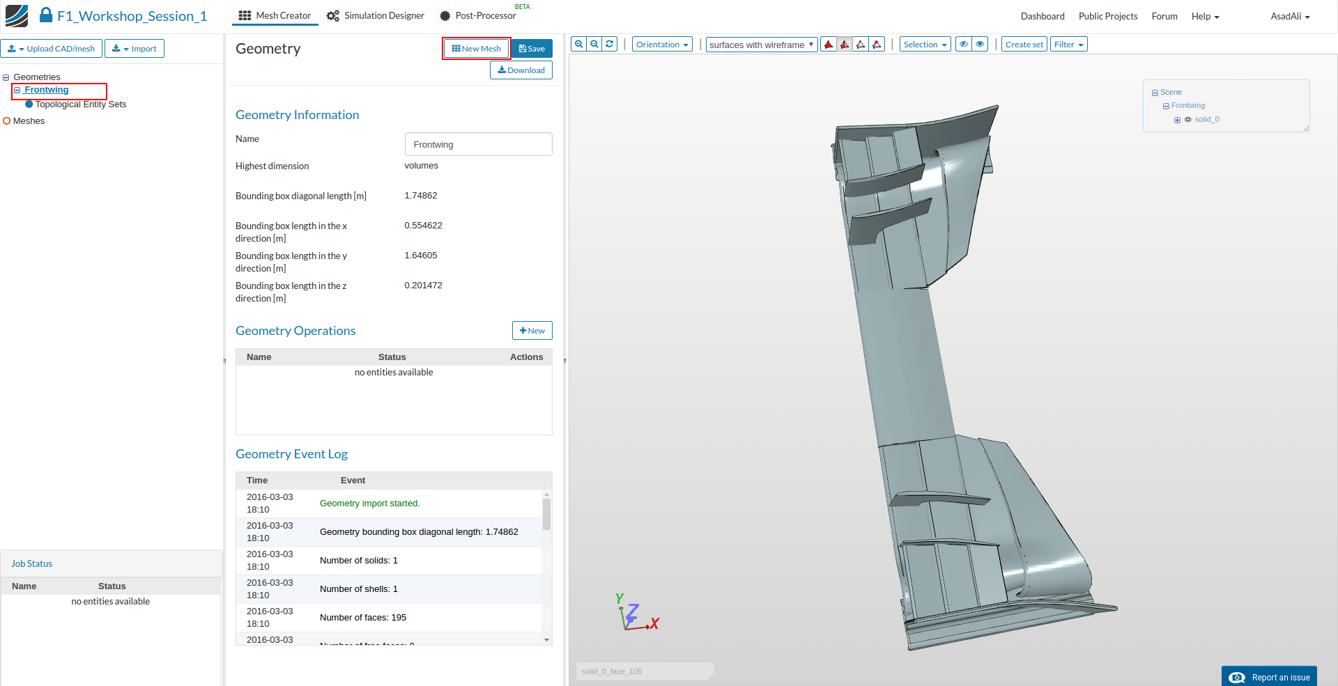
First of all you have to import the geometry into your SimScale workspace. For this, you only have to click on this link. Please note that this can take several minutes. You will be notified when the project has been imported and you will be automatically redirected to the Mesh Creator.
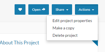
To make this project public, edit the project properties:
and change the visibility to public and save:

Click on the geometry Frontwing in the project tree. This will open an additional column in the middle. Here select the New Mesh to crate a mesh setup for this geometry.
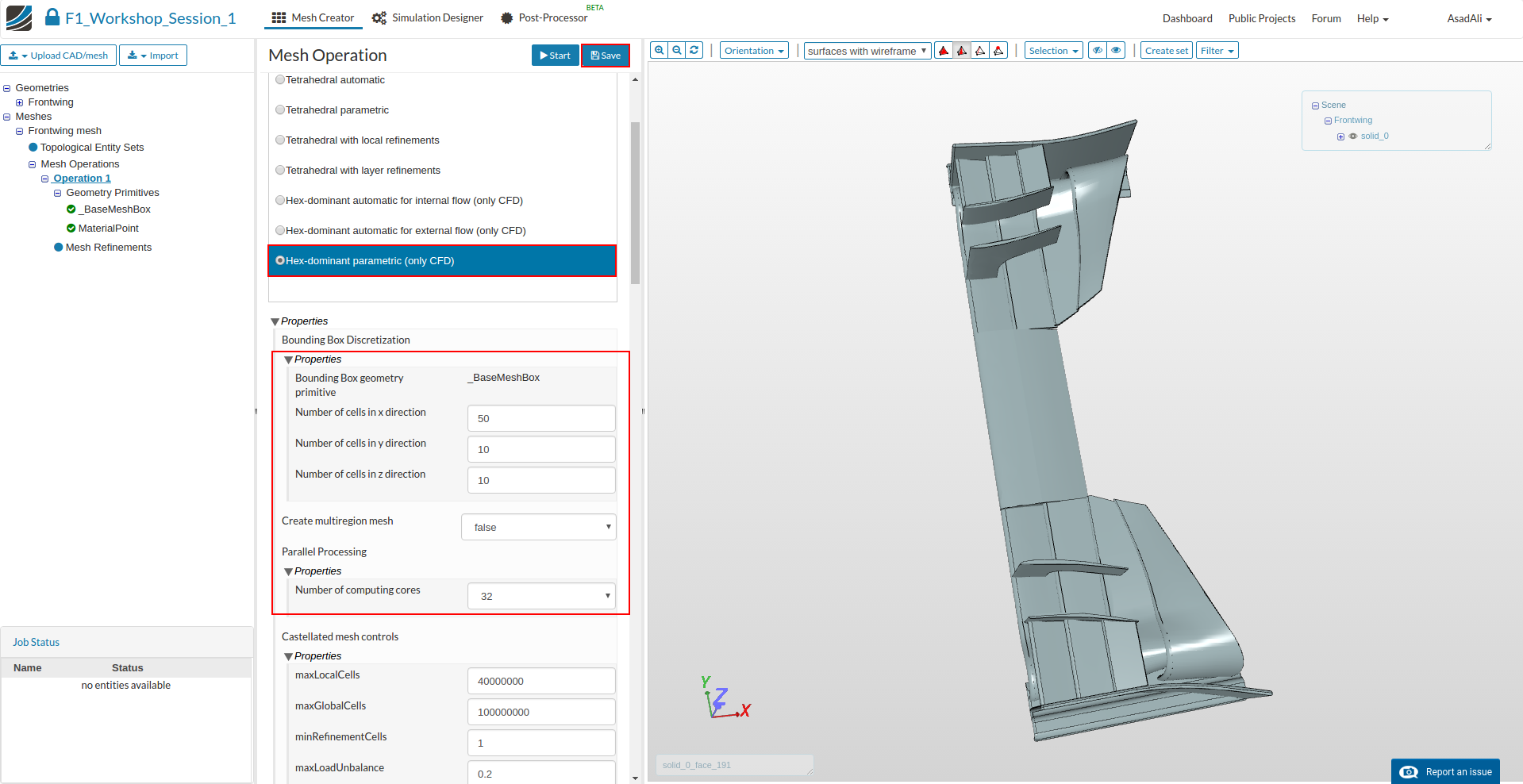
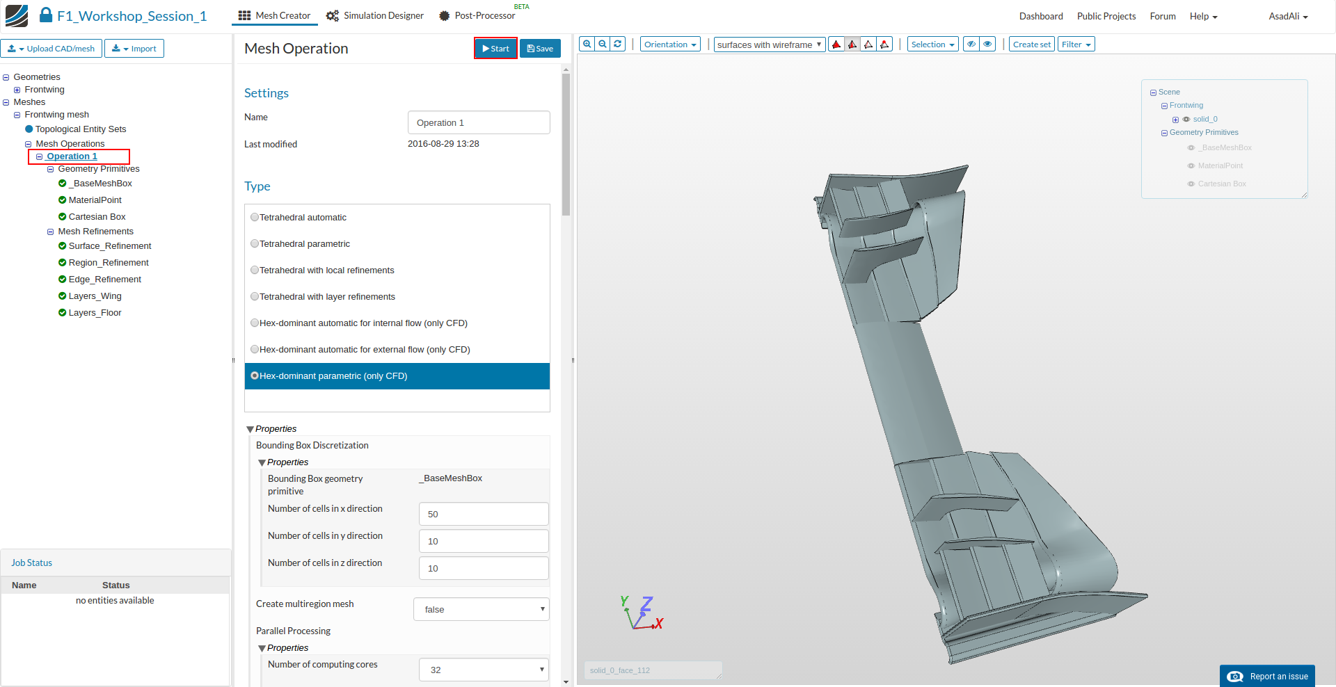
Select the Hex-dominant parametric (only CFD) from the list. In the same panel under Bounding Box Discretization specify the following values for number of cells in each X,Y and Z directions for the BaseMeshBox
- Number of cells in x direction: 50
- Number of cells in y direction: 10
- Number of cells in y direction: 10
- and under ‘Parallel Processing’, the number of processors as : 32
Now click Save to save the selection.
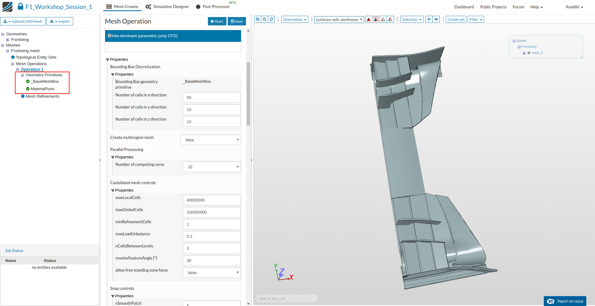
After saving , sub-trees named Geometry Primitives and Mesh Refinements will automatically appear under the default project tree
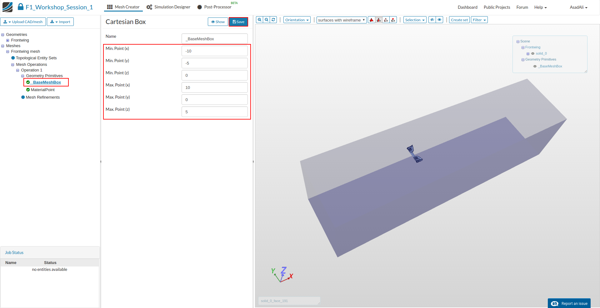
Under Geometry Primitives, click on BaseMeshBox, specify the following values and click on save
- Min. Point (x): -10
- Min. Point (y): -5
- Min. Point (z): 0
- Max. Point (x): 10
- Max. Point (y): 0
- Max. Point (z): 5
Next, click on “material point” and specify the following values:
- Center (x) : -5
- Center (y) : -2
- Center (z) : 1
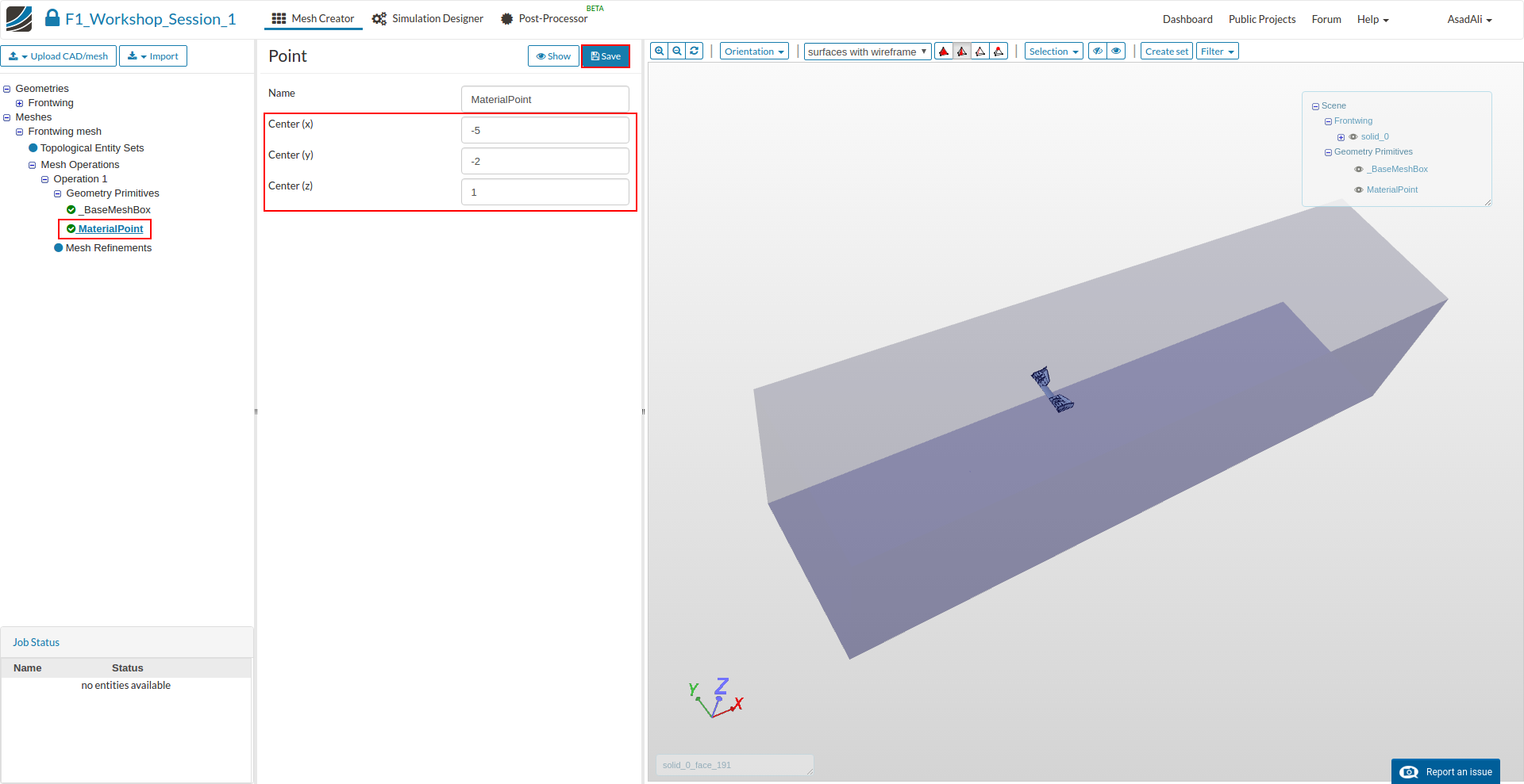
This will place the material point in the space between the Bounding BaseMeshBox and the geometry surfaces. So, this is the confined space that will be meshed.
Next, we create an additional geometry primitive by clicking on Geometry Primitives and then New from the options panel and select type. These will be used to define region refinements later on.
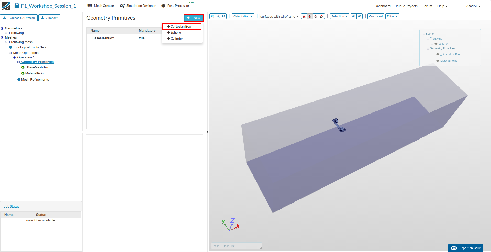
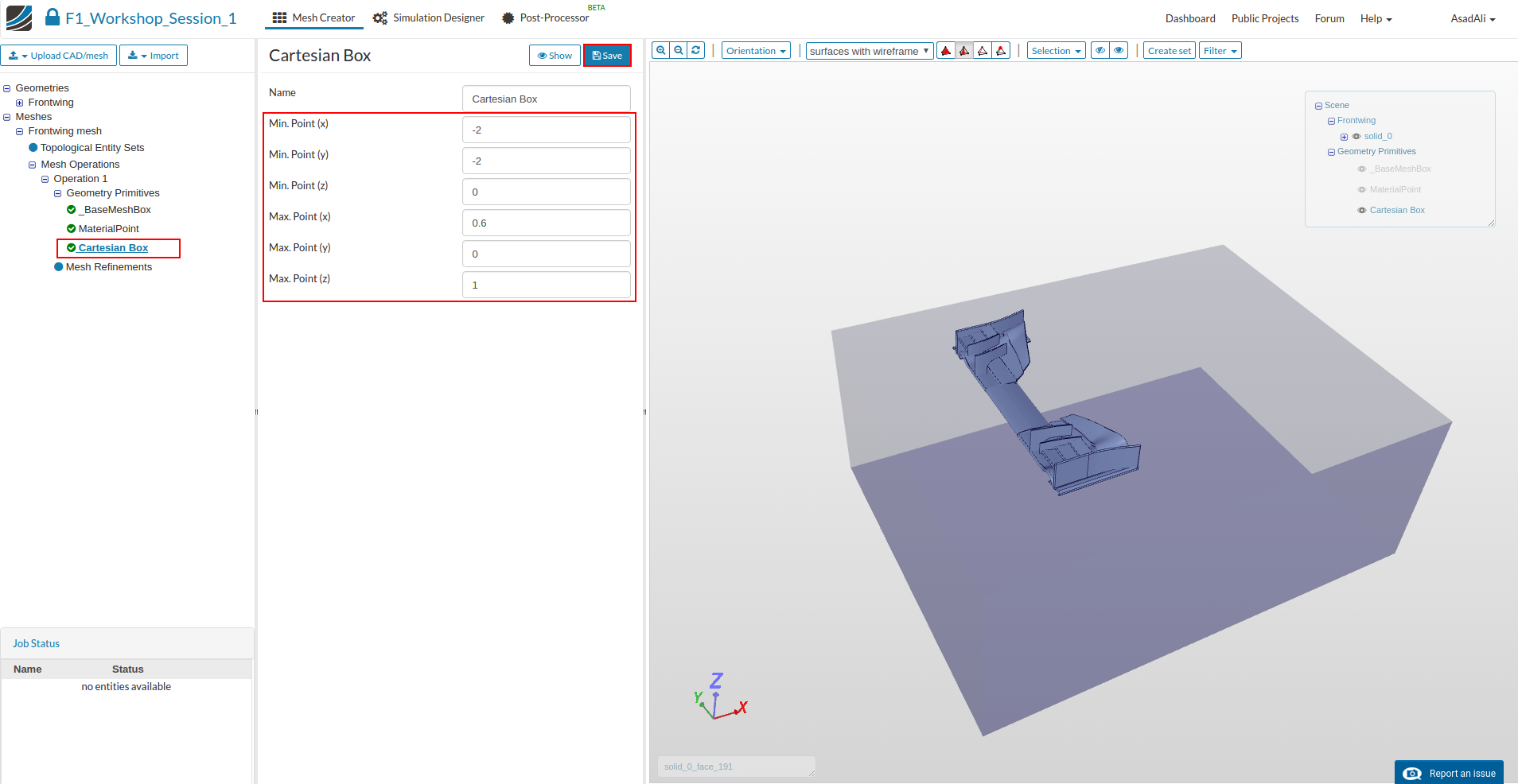
Create a Cartesian Box geometry primitive with following properties:
- Min. Point (x): -2
- Min. Point (y): -2
- Min. Point (z): -0
- Max. Point (x): 0.6
- Max. Point (y): 0
- Max. Point (z): 1
Now, we add the necessary surface, and region refinements for the mesh.
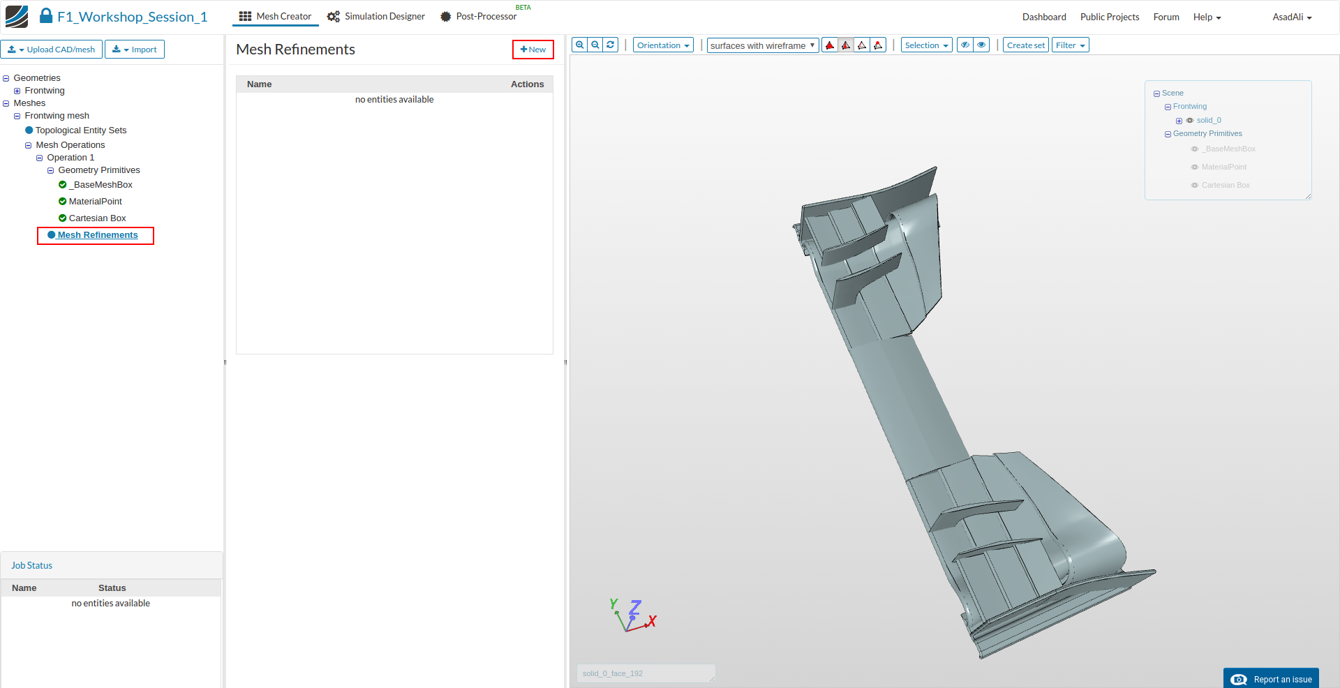
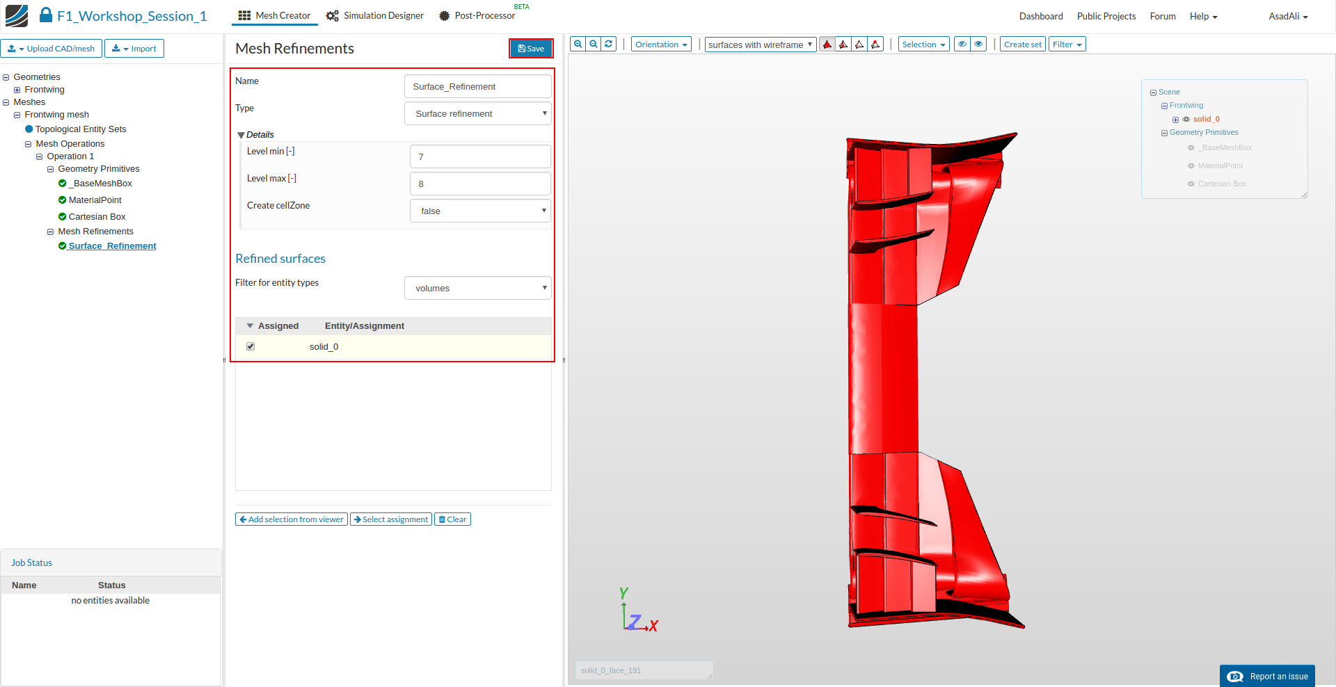
Click on Mesh refinements item in the tree and then click “New” from the options panel to create a new refinement item and adapt the following settings:
- Name: Surface Refinement
- Type: Surface refinement
- Level min: 7
- Level max: 8
Finally, assign it to the whole geometry of the front wing (solid_0)
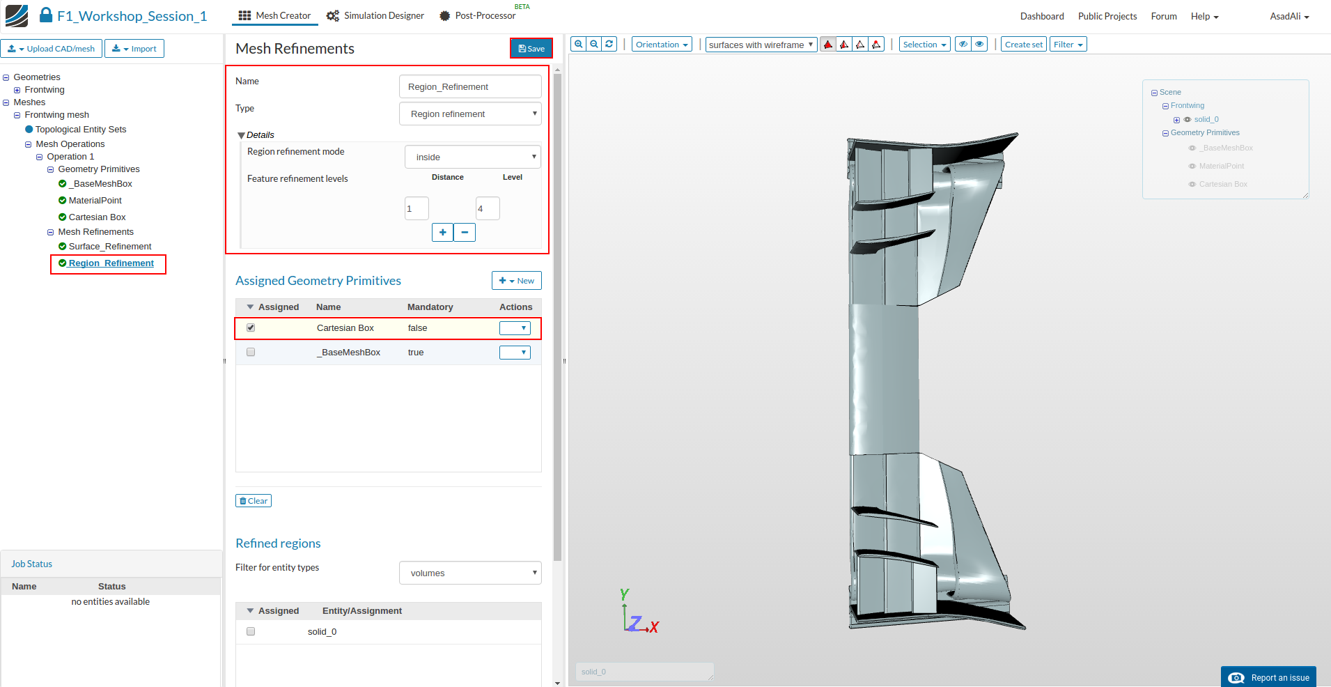
Next we will create a refinement item to create a region refinement around the wing with the following settings:
- Name: Region Refinement
- Type: Region refinement
- Region Refinement mode: inside
- Level: 4
Finally, assign it to the Cartesian Box geometry primitive
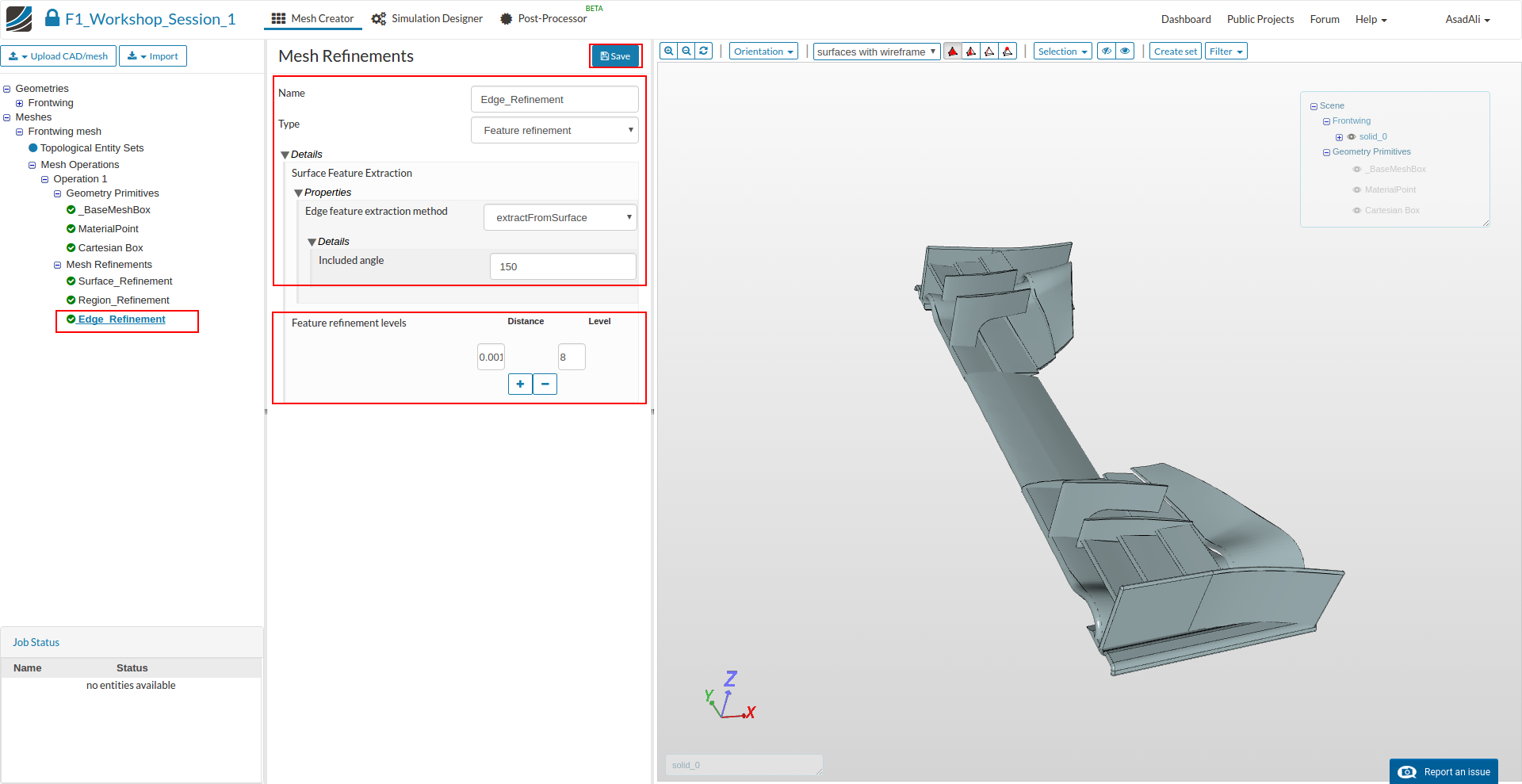
Next, we will create a refinement item to improve the represenation of edges:
- Name: Edge_Refinement
- Type: Feature refinement
- Edge feature extraction method: extractFromSurface
- Include angle: 150
- Distance: 0.001
- Level: 8
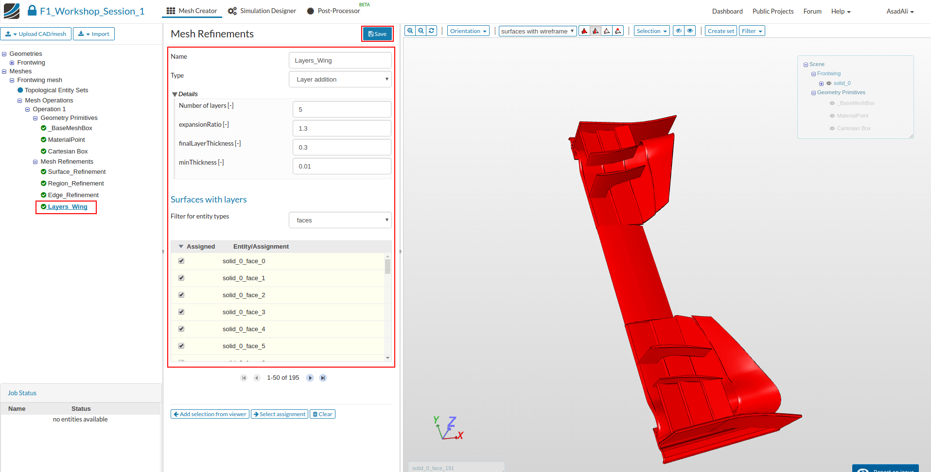
Next, we will add a layer elements to the surface of the front wing:
- Name: Layers_Wing
- Type: Layer addition
- Number of layers [-]: 5
- expansionRatio [-]: 1.3
- finalLayerThickness [-]: 0.3
- minThickness [-]: 0.01
Assign it to all surfaces of the front wing.
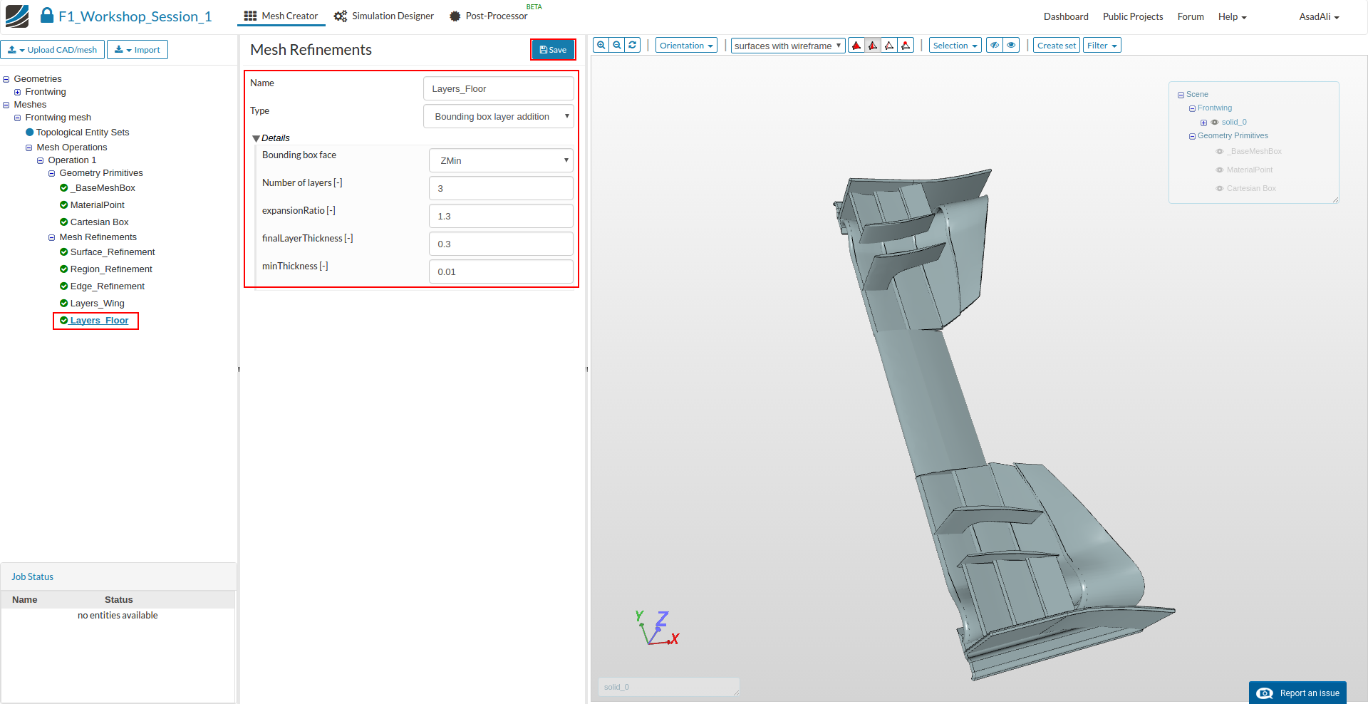
Finally, we will add layer elements to the floor of the base mesh box:
- Name: Layers_Floor
- Type Bounding Box Layer Addition
- Bounding box face: Zmin
- Number of layers [-]: 5
- expansionRatio [-]: 1.3
- finalLayerThickness [-]: 0.3
- minThickness [-]: 0.01
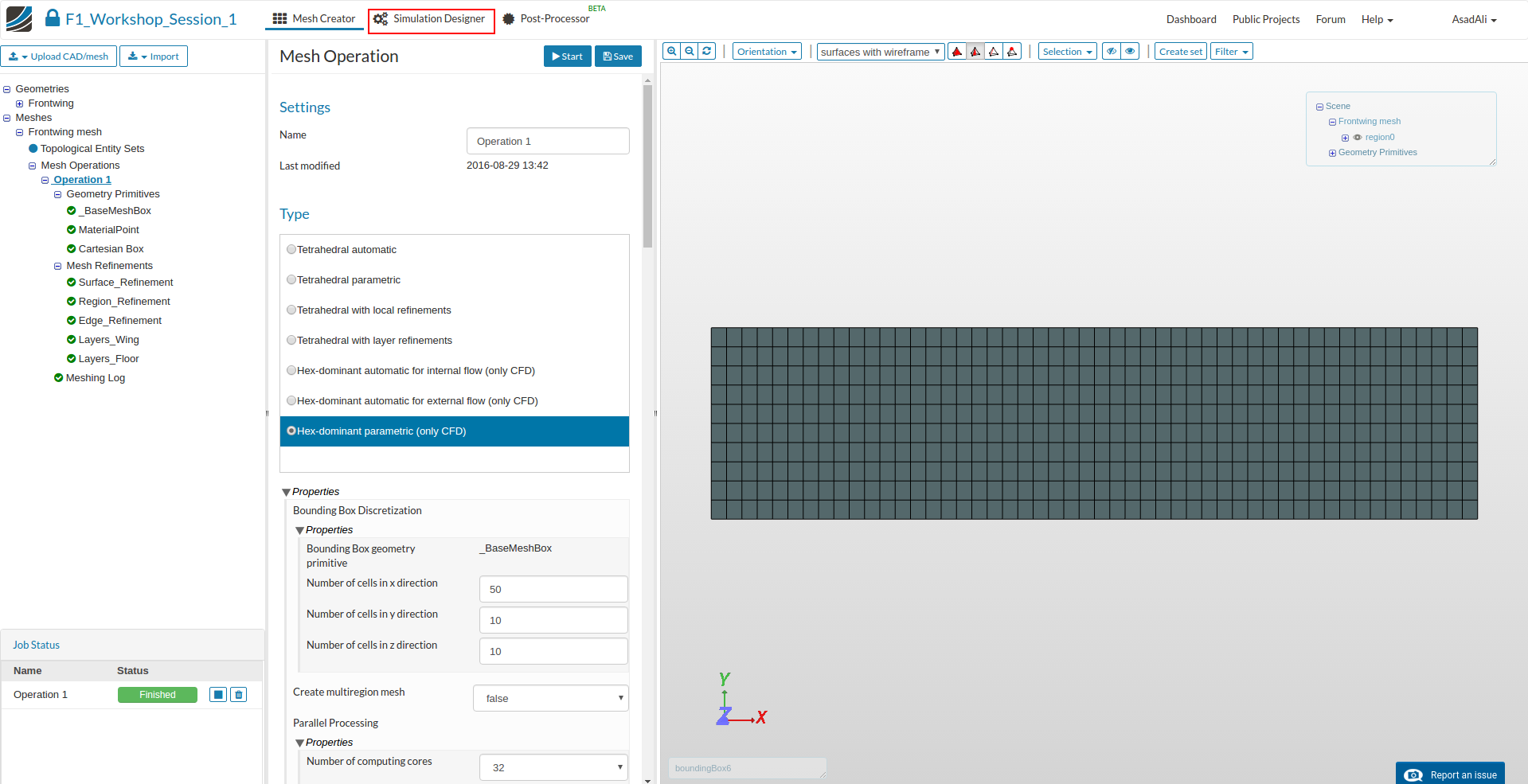
Once done, click save and start the meshing process by clicking on the start button at top. The meshing process will take less than 20 minutes to finish.
Simulation
Click on the** New simulation** button to create a simulation run. This will open an additional column in the middle. Here you can select which kind of simulation you want to run.
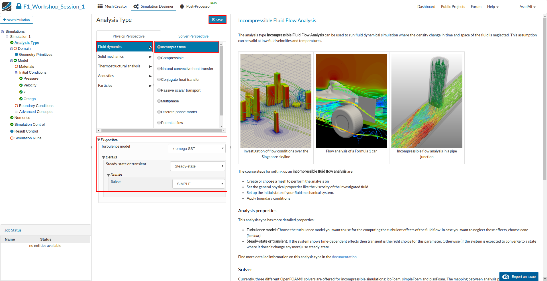
In our case we will run a Fluid dynamics simulation of an incompressible fluid.
Now you can define some additional settings. First of all choose the k-omega SST turbulence model. This is necessary since the airflow around the wing will be highly turbulent. Then choose Steady-State from the drop down field below. This means that we will simulate the stationary flow field. Finally save your settings by clicking the related button at the bottom, which will create additional items in the project tree on the left side.
Going forward, this tree will guide us through all necessary steps. Please note that some of the items are optional.
Next you have to specify which mesh you want to use for your simulation. Click on Domain item in the project tree and select Frontwing mesh from the menu which disappears in the middle column. Don’t forget to save your selection.

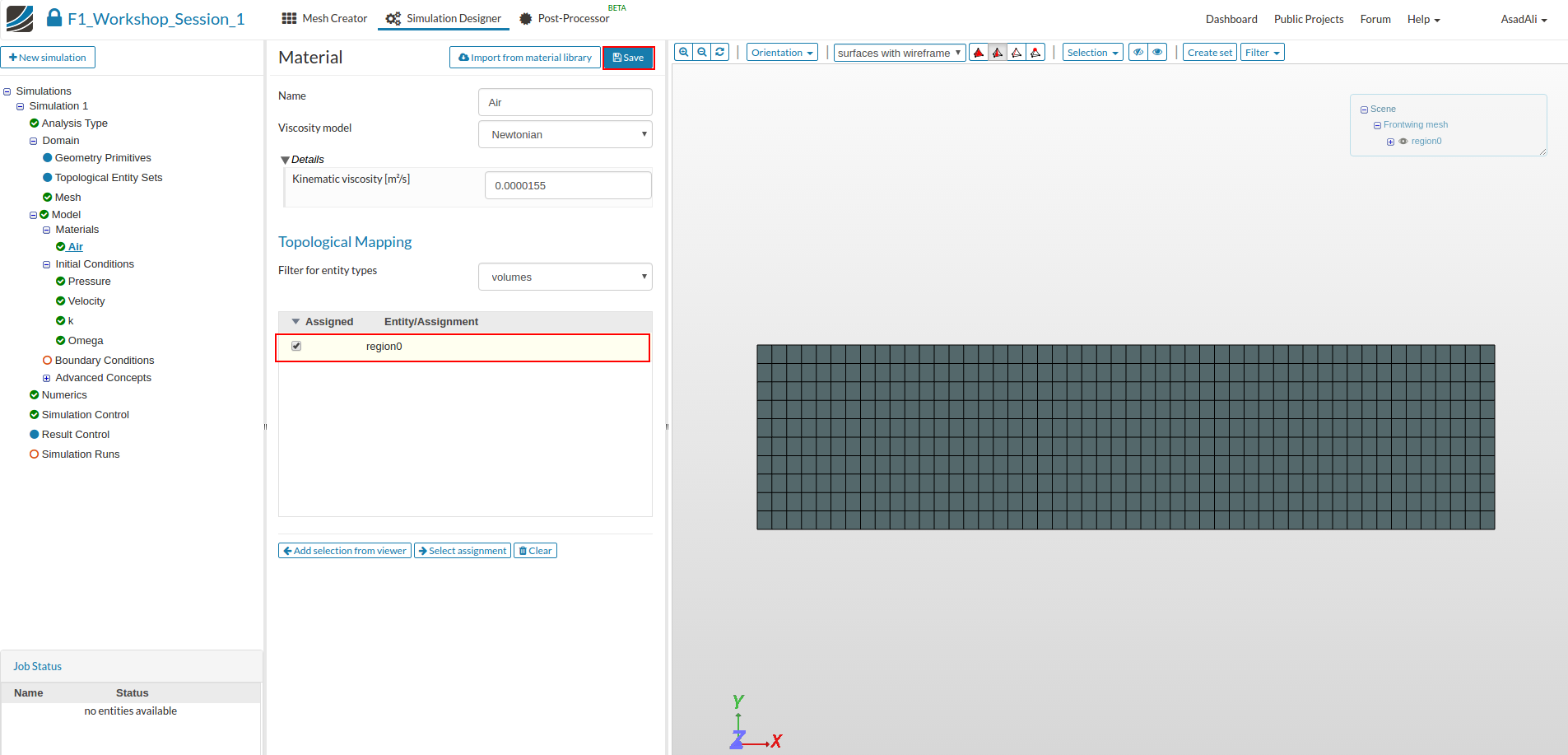
Now we have to specify the Material properties of the fluid by defining the kinematic viscosity. Therefore click on the Materials sub-item in the project tree and click on the New button.
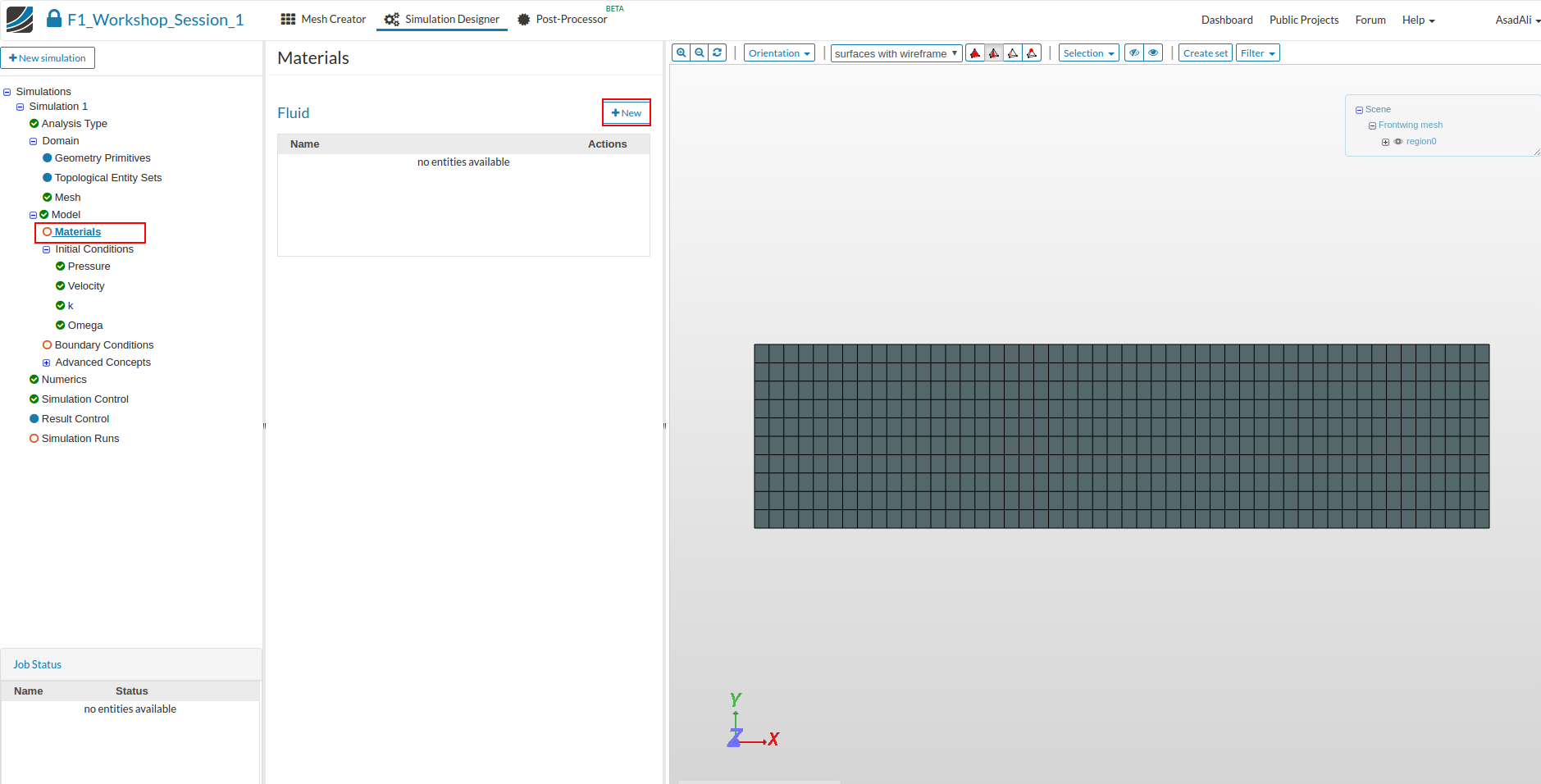
This will open a new middle column windows where you can assign fluids to your mesh. SimScale also comes with a Material library which we will use. Click on the Import from material library button.
Here choose Air from the list on the left side and save your selection.
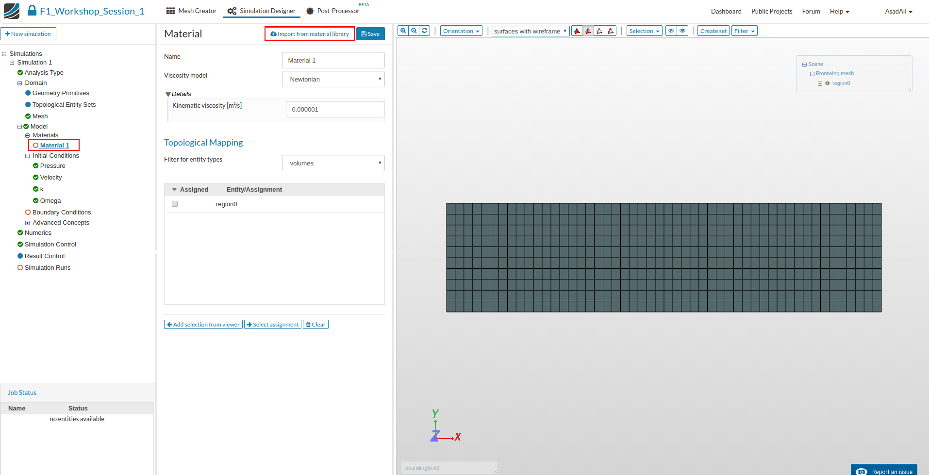
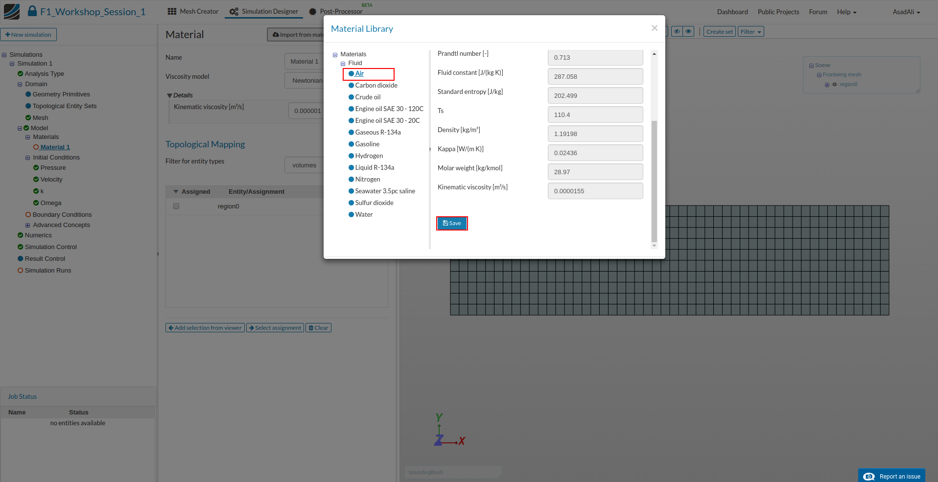
Finally we have to assign which parts of the mesh should be from this material. Please assign the material model to your mesh (region0)
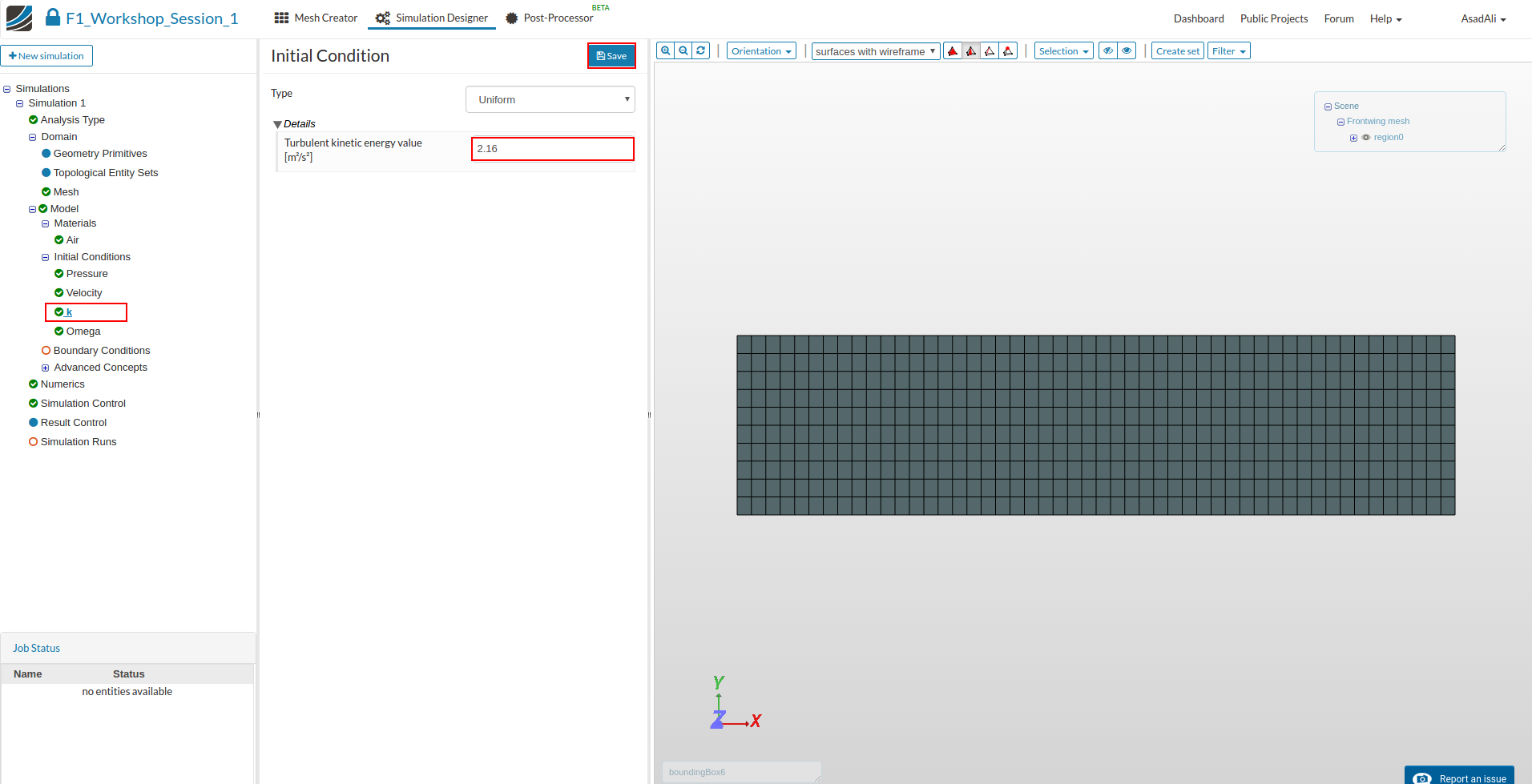
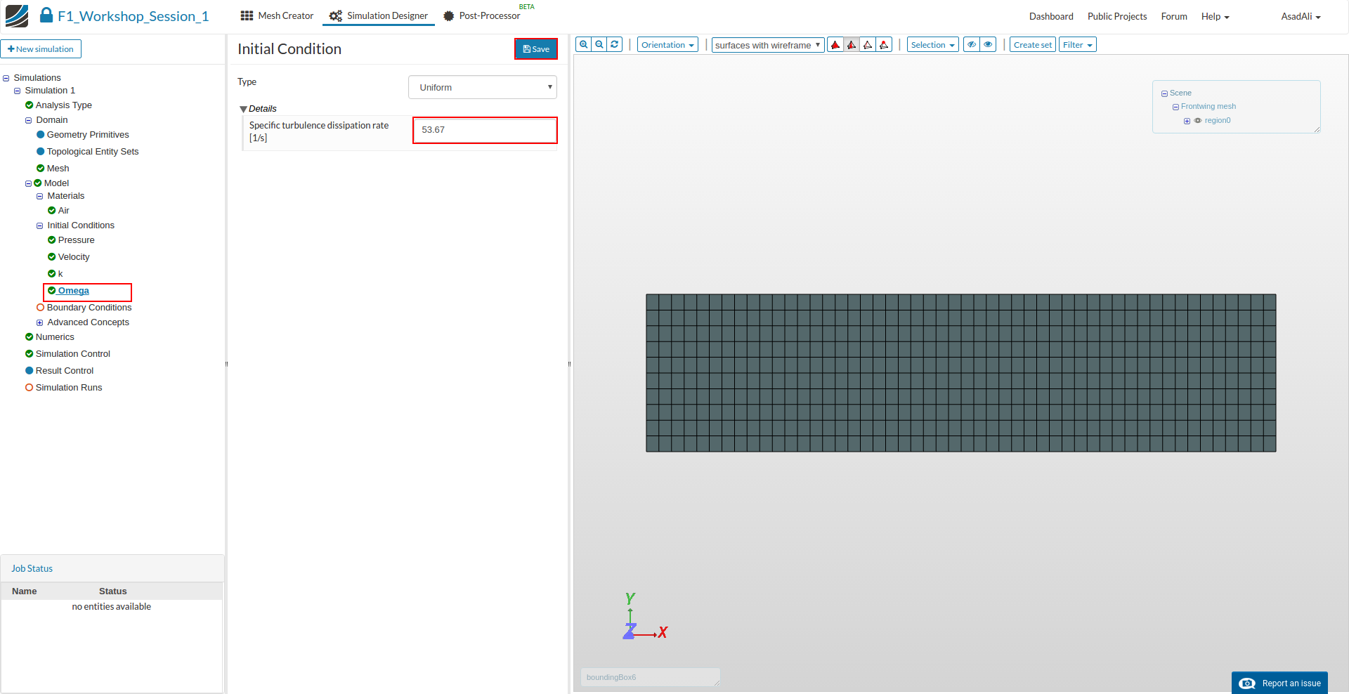
Next we will set up the initial conditions. Click on the Initial Conditions sub-item.The Initial Conditions define the initial values for all physical quantities like pressure, velocity, etc. To understand this you have to keep in mind how engineering simulation actually works: Since the mathematical equations which describe the motion of fluids can only be solved numerically, the solver needs an initial solution to iterate. In some special cases it can be necessary to adapt this in order to make the simulation more stable.
The initial conditions for velocity and pressure does not need to be modified in general.
In contrast to that it is quite important to use the right turbulence model paramters k and omega. They can be calculated following this instructions:
Please change the initial value of k to 2.16
Next change the initial value of omega to 53.67
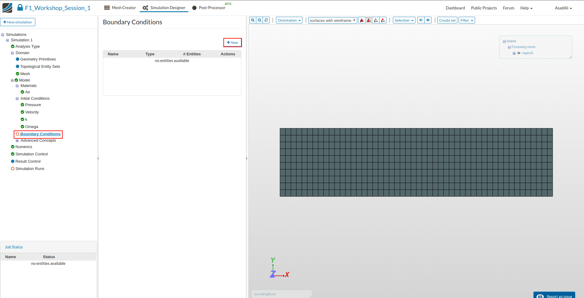
Now you can start to specify the physical behavior of the front wing and its interaction with the environment by defining the Boundary Conditions for all faces of the mesh.
Click on the Boundary Condition item in the project tree which will again open a new column in the middle of the windows. Here you can see an overview of all boundary conditions which are applied to your mesh. To add a new boundary condition, please click on the related button at the bottom of the middle column.
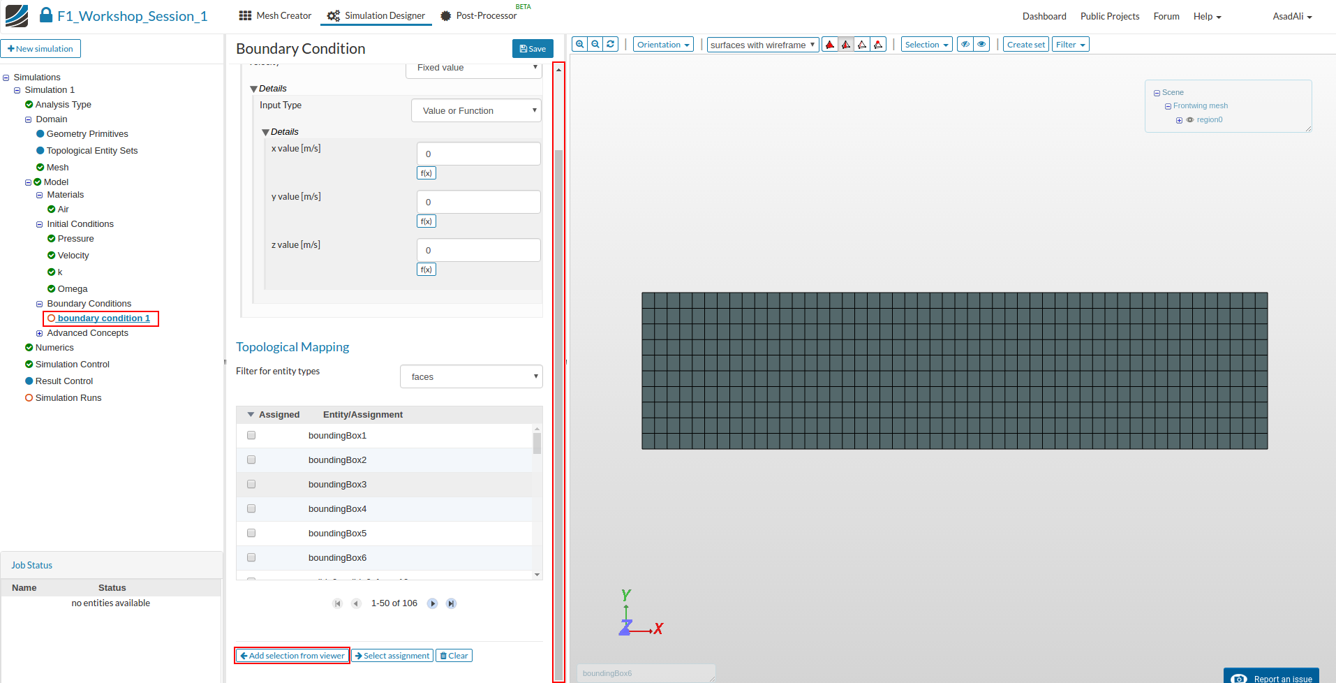
This will add a sub-item to the project list and open again a new window where you can define the boundary condition. Here you can define a name for the boundary condition, choose the type and assign it to faces by using the list below.
It is also possible and recommended to select the faces which you want to assign to the boundary condition graphically. Therefore you have to select the faces in the 3D model window on the left side by clicking on them with the left mouse button; to add them to the list, just click on the Add selection from Viewer button in the middle column.
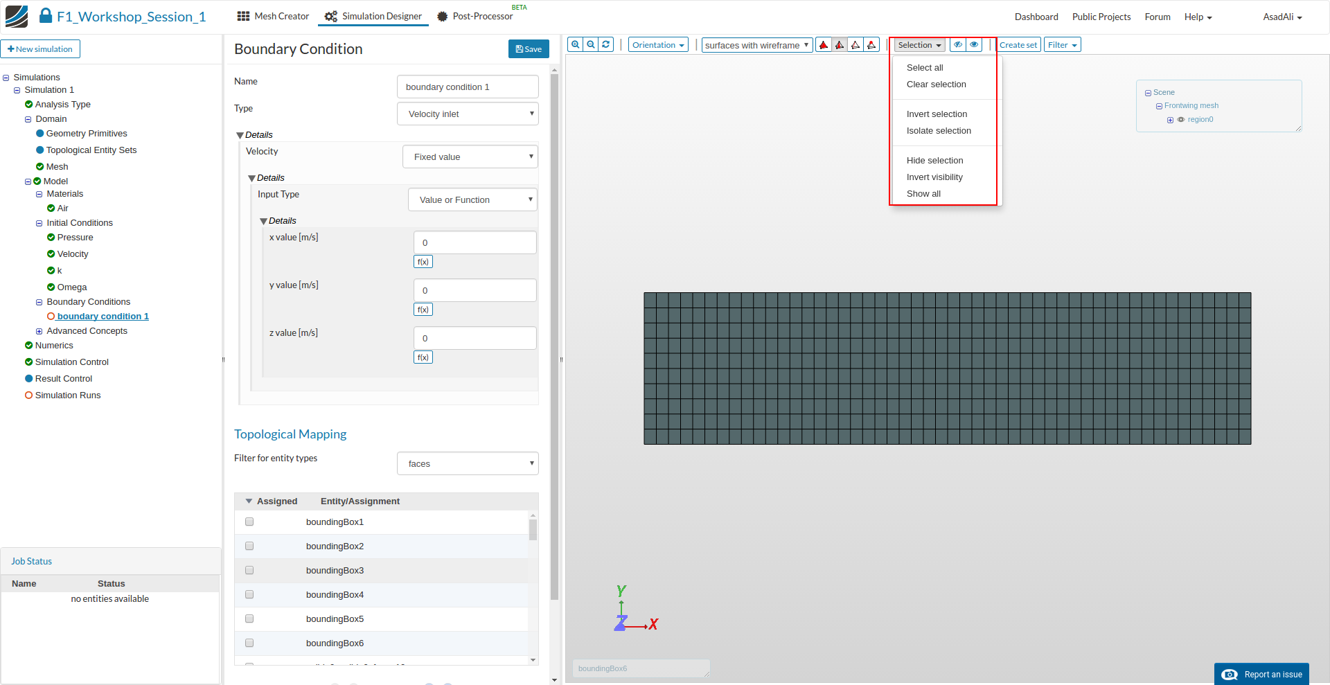
Since the full mesh domain is displayed, it is necessary to hide these faces in order to be able to select the inner faces. For this, just select the faces you want to hide and click on the Hide Selection button from the drop down menu on top of the 3D model windows. Note that you can unselect faces by re-clicking on them.
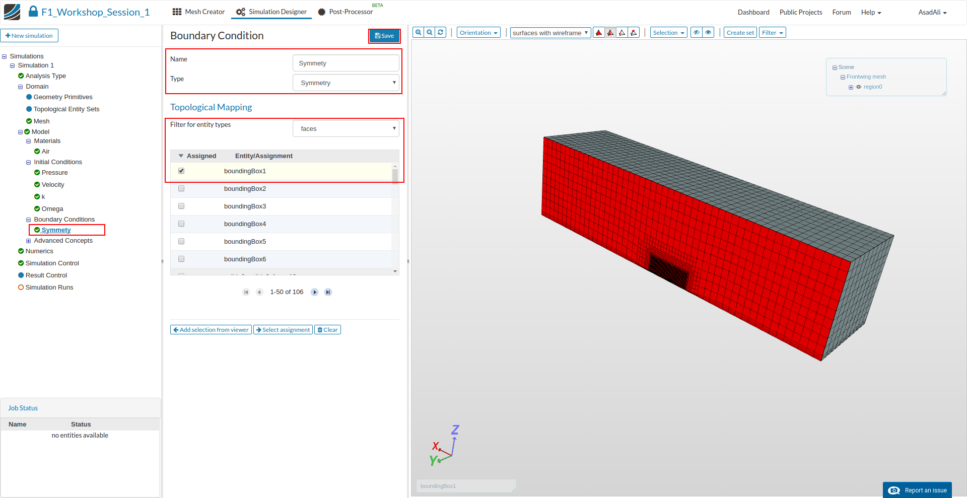
Symmetry
This boundary condition is required because we are using a half model of the front wing. Please select Symmetry as the type and the symmetry plane(boundingBox1) which intersects with the front wing.
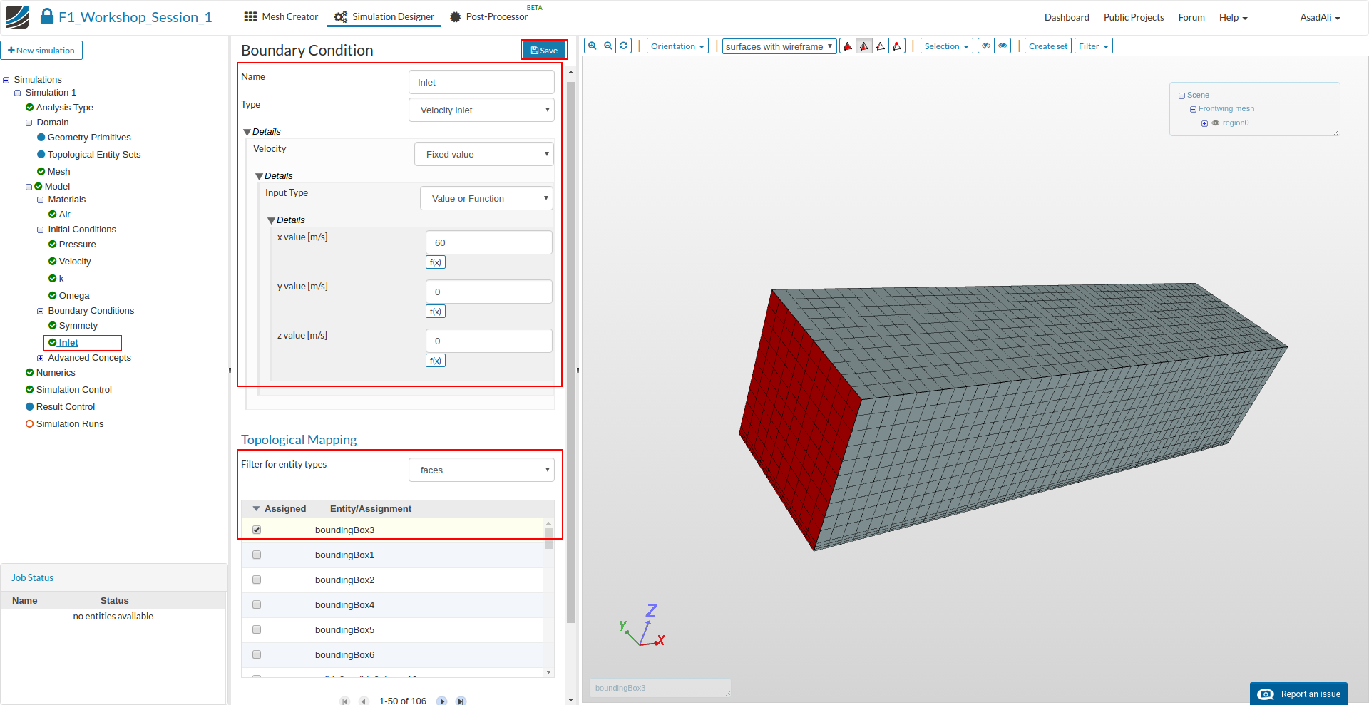
Inlet
This boundary conditions is necessary to define where the flow should enter the domain. Please select Velocity inlet with Fixed value and Value or Function as the input type with a velocity of 60 m/s in x-directon.
Now select the face in front on the front wing (boundingBox3)
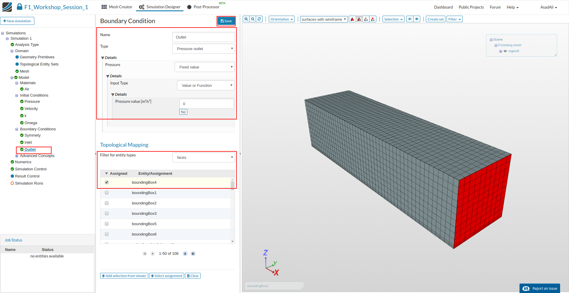
Outlet
This boundary condition is necessary to define where the flow should leave the domain.
Please select Pressure outlet with Fixed value and Value or Function as the input type with zero pressure.
Now select the face behind the front wing (boundingBox4)
Slip-Walls
As already discussed, this boundary conditions will reduce the interaction of the other surrounding walls. It is necessary because these walls do not exist in reality.
Please select Wall as the type and Slip for Velocity and Wall function for the wall treatment. Now select boundingBox6 and boundingBox2, and add them to the list of faces.

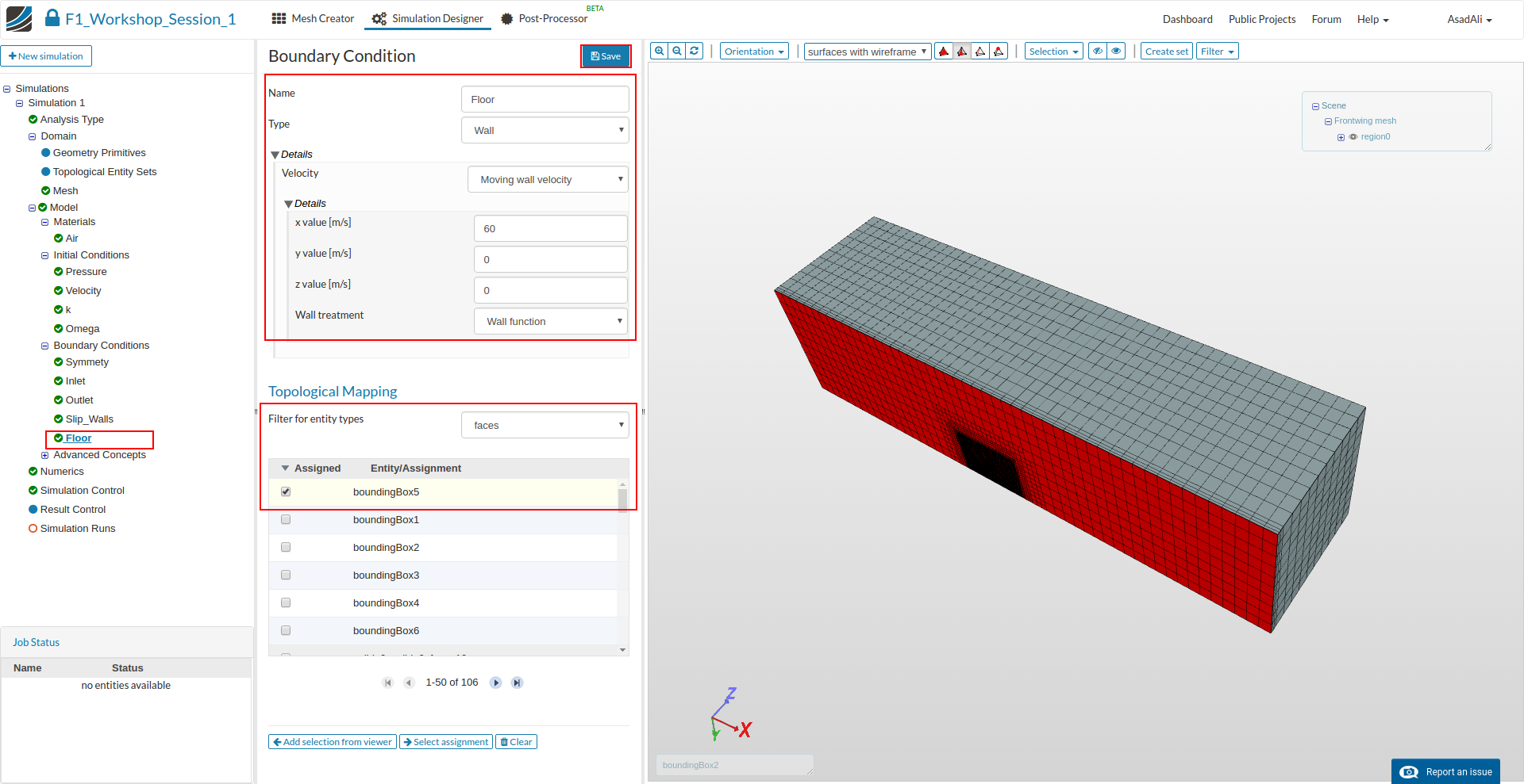
Floor
There is no relative motion between the air and the floor since the car is driving through our domain. We will, therefore, apply a wall velocity on the lower surrounding wall.
Please select Wall as the type and Moving wall velocity as the sub-type. Next, apply a velocity of 60 m/s in x-direction and apply in on boundingBox5.
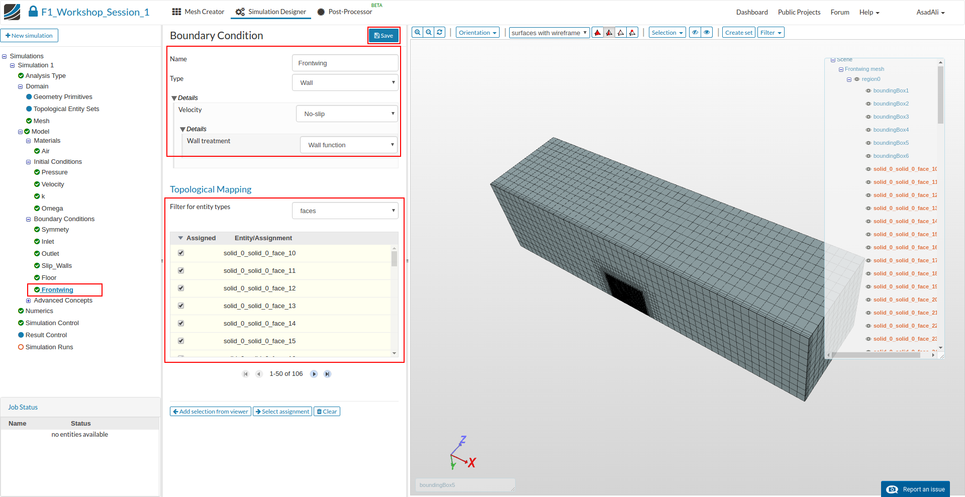
Frontwing
Finally we will apply the boundary condition to the front wing.
Please select Wall as the type and No-Slip for Velocity and Wall function for the wall treatment and assign it to all faces of the front wing
Now we have to modify some of the numerical settings. This is not absolutely necessary but it will help to reduce the simulation time and make it more stable. Click on the Numerics items in the tree and change the settings and values according to the image below (Please note that you have scroll down).

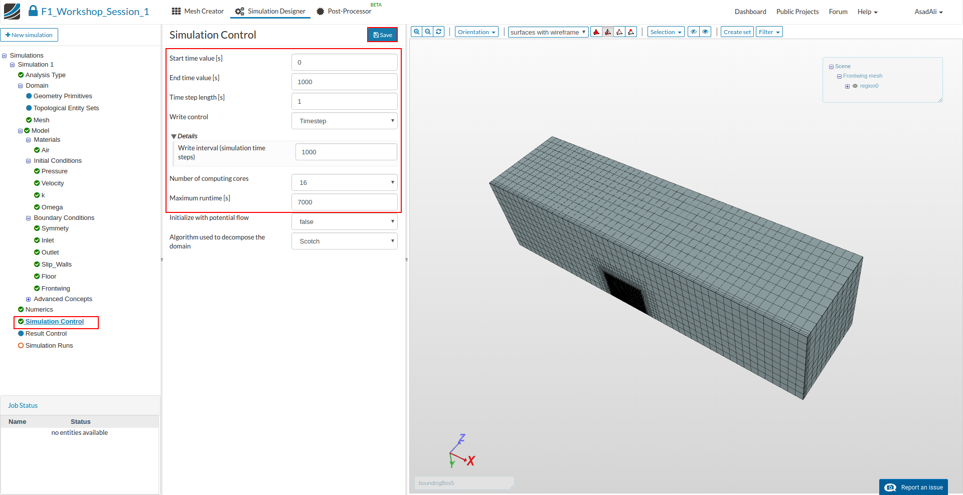
Click on the Simulation Control item in the project tree to specify how fast and accurate you want the simulation to be computed.
Choose 0 as the Start time value and 1000 as the end time value. The time step length must be 1 and the write intervall 1000. Finally, choose 16 computing cores from the drop down menu and define a maximum runtime of 7200 seconds (this is the time after the simulation will automatically be aborted).
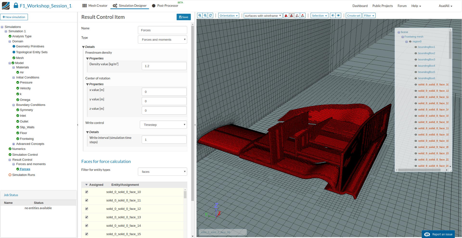
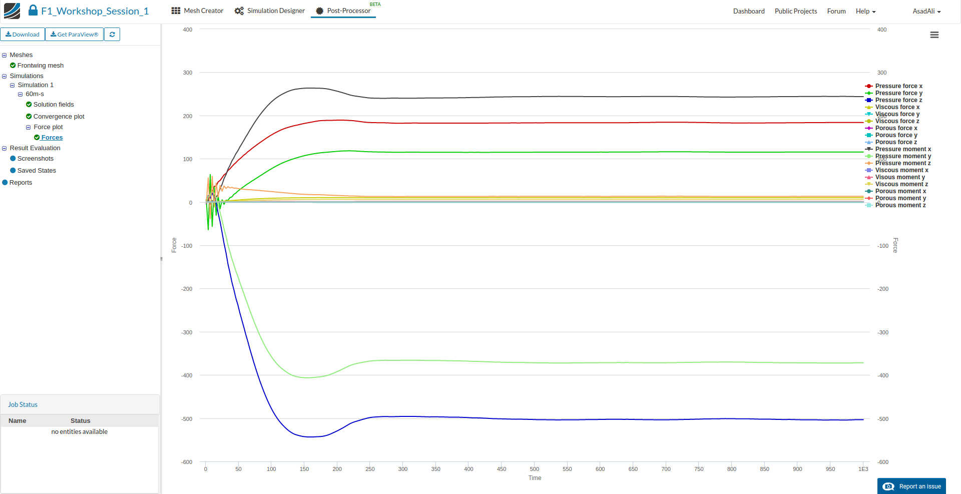
To “measure” the lift and drag force of the front wing we have to add Result Control item. Click on the corresponding item in the project tree and click on the New against the “Forces and moments” item button.

Choose Forces and moments as a type, define a Density of 1.2 kg/m³ and (0 0 0) as the Center of rotation. Skip the remainingsettings and add all surfaces of the front wing to the surface list (workflow according to the front wing boundary condition)
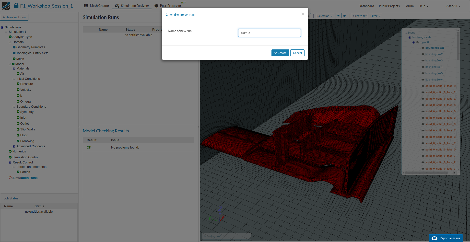
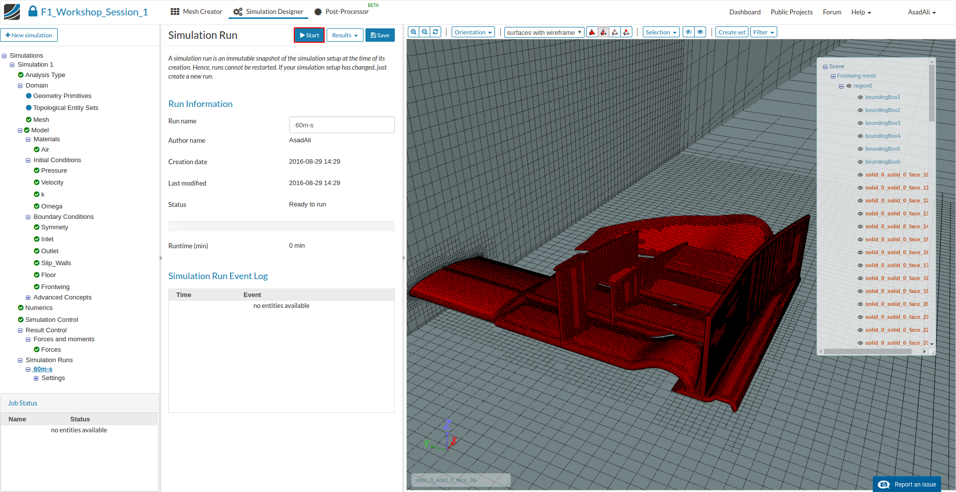
To start the simulation, click on the Simulation Run item in the tree and click on the Create new run button at the bottom of the middle column menu. This will create a snapshot of your simulation settings as a new sub-item.
Post Processing
You will be notified when your simulation run is finished. Please switch to the post-processing envoirment by clicking the related tab in the main ribbon bar
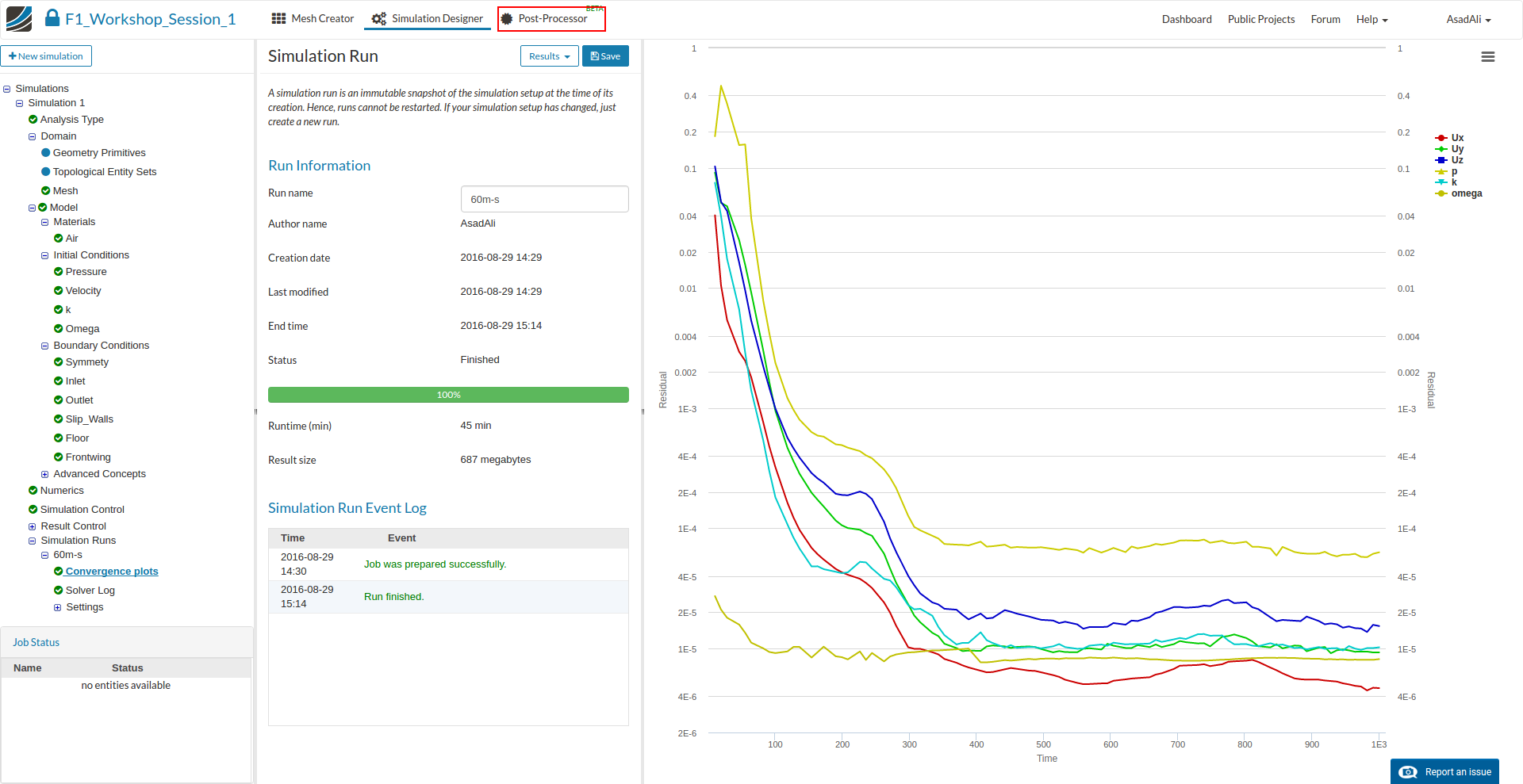
Here you can investigate the forces which are generated by the front wing for every single iteration of the simulation.
You can also analyze the 3d simulation results by clicking the Solution fields item in the post processing tree. Please follow this video tutorial if you are interested in 3d result visualization:

Congratulations, you have completed the Homework of Session 1 and can now move on to Session 2:
