Tutorial Updated 2018-02
Recording

Introduction
The CFD Master Class: Session 1 explores the methodology of correctly defining the first cell wall distance, and its effect on results obtained using the wall modelling technique and assessing the resulting near wall velocity.
During this session we shall explore the concept of Y+, how to predict the wall distance Y from an approximated Y+ and how to correct your mesh using results obtained from the simulation.
The first part of this exercise will be setting up the base mesh, then duplicating it to vary the properties of a layer refinement. The second part will be setting up the simulation with appropriate settings and result control items in order to properly analyse the results. The final part will be dedicated to understanding the results and drawing conclusions upon correct and incorrect settings and their impacts on results.
Boundary Layer Modelling
When analysing flow in contact with a wall, we must ensure that the boundary layer is correctly solved to ensure that results are accurate. The effects of not correctly solving the boundary layer can vary depending upon the scenario, skin friction is likely to alter effecting drag results and flow separation is likely to alter if the boundary layer isn’t properly solved.
In SimScale there are two techniques to solve the wall, we can either fully resolve the boundary layer, requiring many cells, and making the simulation computationally expensive. The other option is to model the wall starting somewhere in the log-law region. This reduces the requirement for many fine cells at the walls. Since this model starts in the log-law region it is necessary to analyse Y+ to ensure that the first cell does, in fact, end in the log region, with the SimScale documentation recommending the value to be between 30 and 200.
This session concentrates on correctly defining mesh layers iteratively based upon results. To do this we will be looking at the quality of the velocity profile as well as Y+ results.
Import Project
To start this exercise, please import the project into your workbench by clicking on the link below:
Project Link: SimScale Login
Mesh Generation
Select Airfoil-NACA0012 in the Navigator on the left side of your screen and click New Mesh. A new mesh will be added to the Navigator.
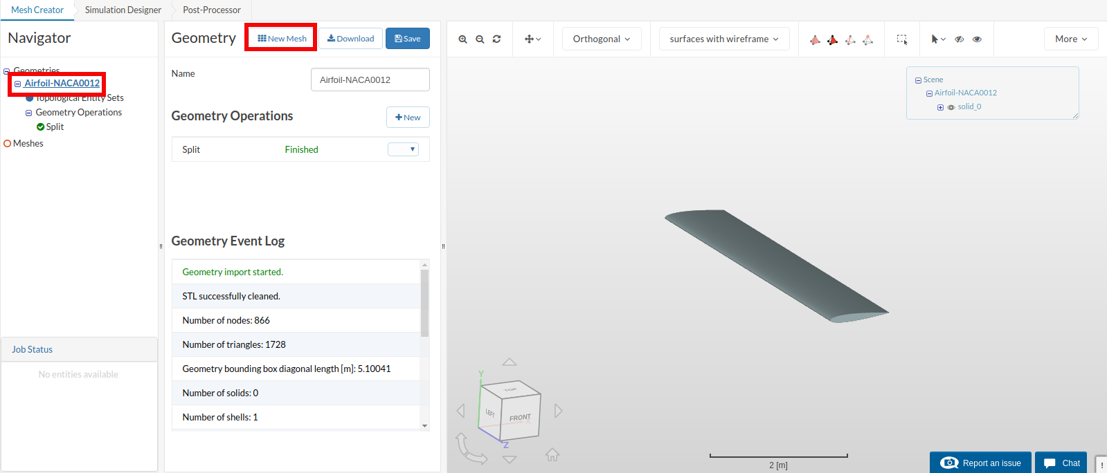
Figure 1: Creating new mesh
Under Airfoil-NACA0012-mesh, add an operation and select Hex-Dominant parametric (only CFD).
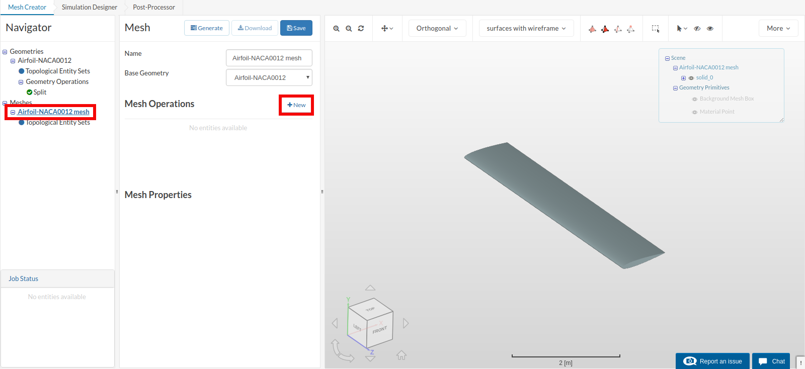
Figure 2: Creating new Operation
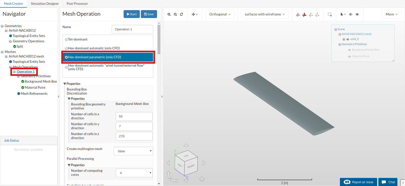
Figure 3: Select Mesh Type as Hex-Dominant Parametric
On the same panel, it is necessary to make a few changes to the default setting, by hovering over each setting you can get a detailed explanation of what the setting is altering.
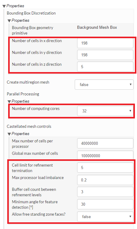
Figure 4: Alter Bounding Box, Parallel Processing and Castellated Mesh Control properties
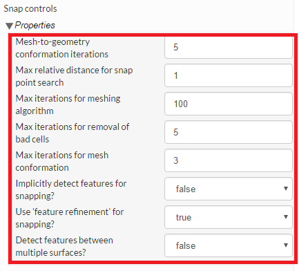
Figure 5: Alter Snap Control properties.
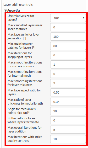
Figure 6: Alter Layer Adding properties.
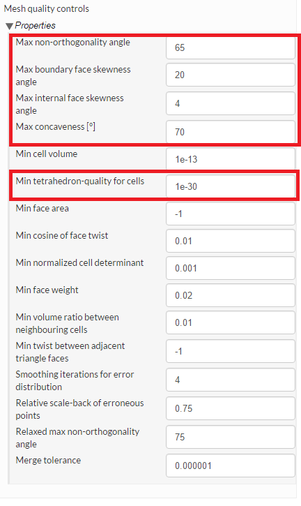
Figure 7: Alter Mesh Quality Control properties.
Press save to commit the changes.
In the Navigator Tree, select the Background Mesh, located under Geometry Primitives.
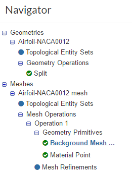
Figure 8: Select Background Mesh from the Node Tree
The Background Mesh defines how large the external domain around the airfoil is, change the settings to match those pictured below.
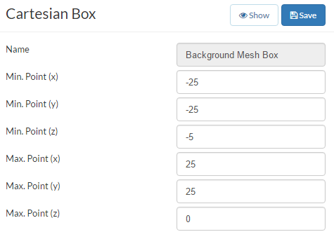
Figure 9: Example settings required to correctly define Bounding Box.
The next item to address is to correctly define the material point. The material point tells the mesh where the fluid region is. In this case, we are performing an external mesh and therefore the material point is required to be outside the airfoil geometry but inside the background mesh. You can alter the setting to match that depicted below. The Material Point can be found in the Node Tree below Background Mesh.
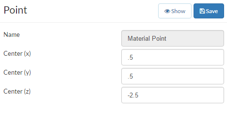
Figure 10: Example settings required to correctly define Material Point.
Following these primitive settings, we need to think about how to refine the mesh in key areas. One method of refinement, Region Refinement, requires geometry primitive volumes to refine cells contained within the primitive. These refinements allow the physics to be better captured in the areas of interest, without the need to globally refine the mesh causing many cells to be created where they are not needed. Therefore, we now need to define these primitives, starting from the largest primitive to the smallest.
A large cylinder needs to be defined around the aerofoil to add a coarse refinement, followed by a smaller one to give a more targeted, finer refinement around the aerofoil. Following this, we shall define long thin primitives on the leading and trailing edges of the aerofoil.
Start by clicking on the Geometry Primitives item in the Navigation Tree and then +New drop down. From the options select Cylinder. Rename it to the Cylinder-outer, set the parameters as shown, and click Save.
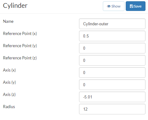
Figure 11: Settings required to define the Cylinder-Outer.
Click Show at the top of the panel to see Cylinder-outer in the display area.
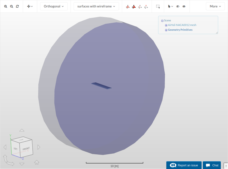
Figure 12: Cylinder created by Cylinder-Outer.
Create another geometry primitive called Cylinder-Inner and set it up with the following parameters.
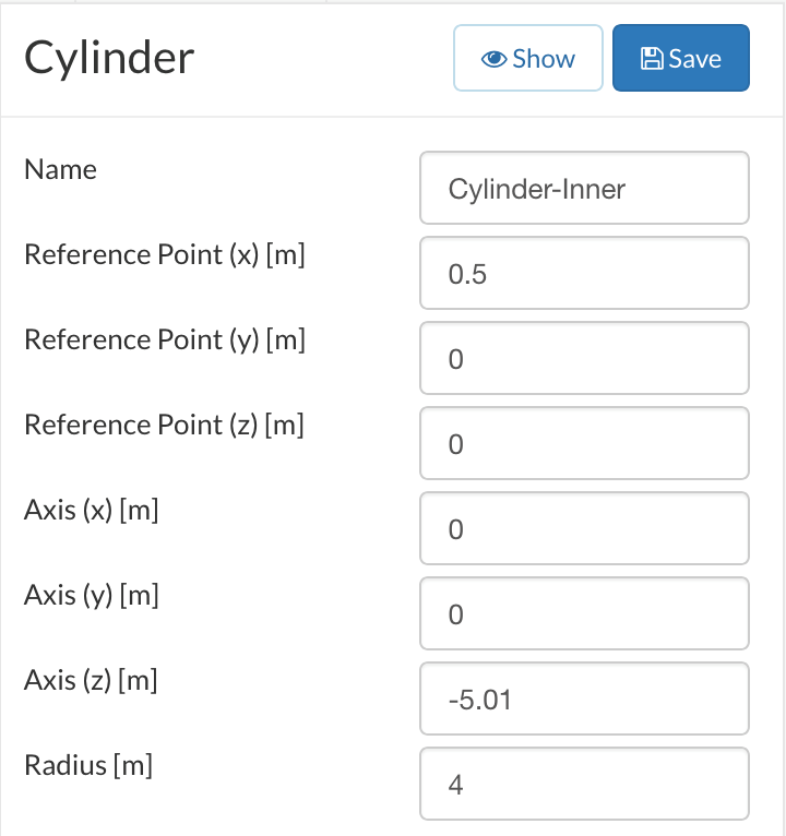
Figure 13: Settings required to define the Cylinder-Inner.
This cylinder will be used to create a higher level of refinement around the aerofoil. It can be visualised along with the Cylinder-Outer by showing them both in the tree.
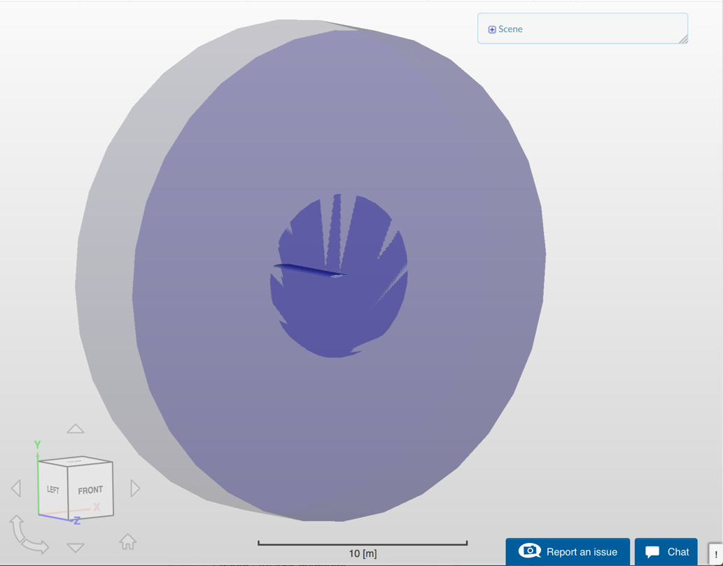
Figure 14: Cylinder created by Cylinder-Inner, compared to Cylinder-Outer.
The next primitive will be a Cartesian box, encapsulating the aerofoil. This allows for an even higher refinement in the region of the airfoil.
Create a new Geometry Primitive using Cartesian Box, rename the primitive to Airfoil-Region. Set the parameters to match the following.
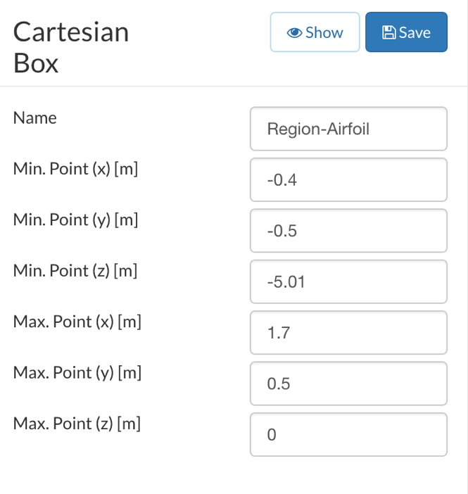
Figure 15: Settings required to define the Region-Airfoil.
The box should fit tightly around the airfoil.

Figure 16: Cartesian Box created by Region-Airfoil.
Using the same techniques, use the following parameters to create the remaining cylindrical geometry primitives.
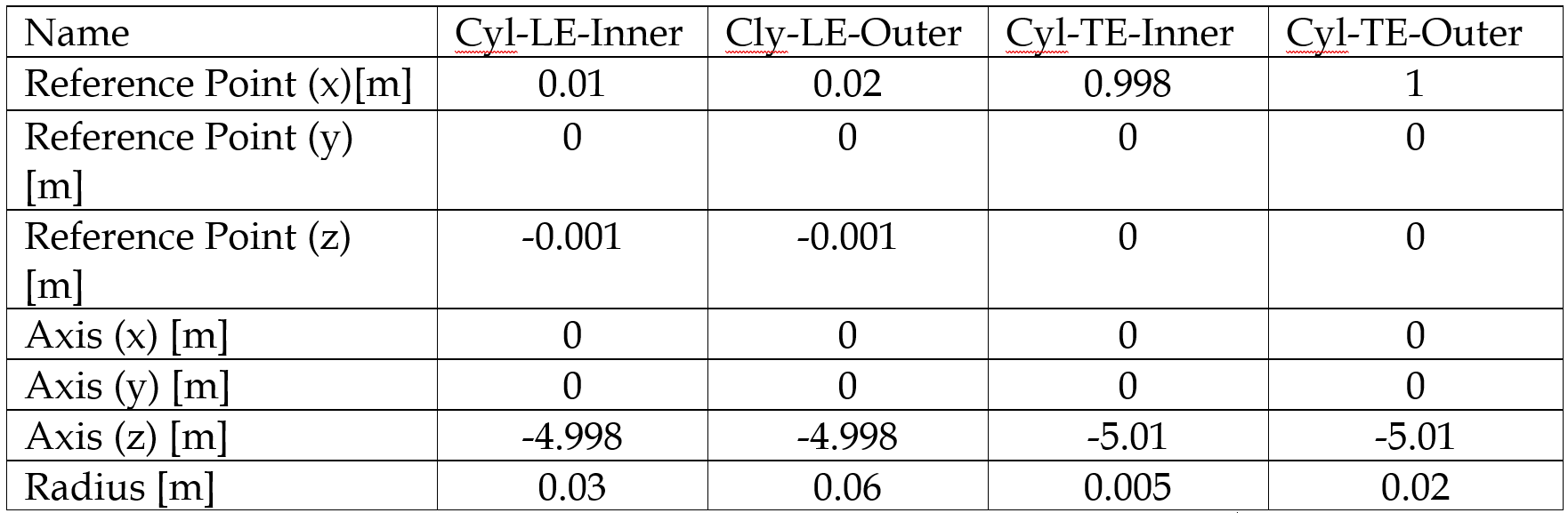
Table 1: Settings for additional cylindrical Geometry Primitives.

Figure 17: Side view of further cylindrical primitives.
At this point, all geometry primitives should be defined, and available for them to be used in the mesh refinement setup, check your primitives off against this list before you move on.
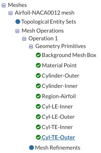
Figure 18: List of primitives in the navigation tree.
Now all the require primitives are defined we move onto the next task in the meshing stage, defining refinements. Refinements are available in many forms, the most common being surface, region and layer inflations refinements.
Starting with the airfoil surface refinement, navigate to the Mesh Refinement node and in the top right of the panel click +New or right-click on the node text and Add Mesh Refinement.
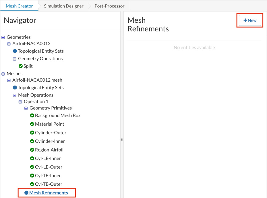
Figure 19: Click +New or right click Mesh Refinements in the node tree for Add Mesh
Once a new refinement has been created change the Type and Name to Surface Refinement and alter the min and max Level both to 6. Finally, in the graphical viewer, change selection type to volume and select the Airfoil.
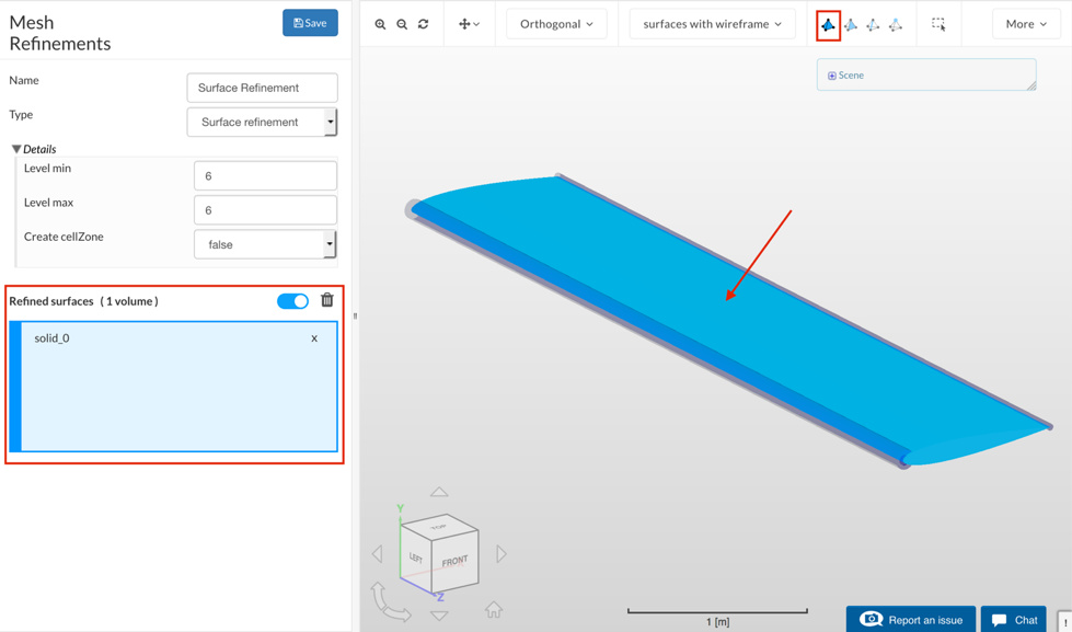
Figure 20: Shows settings and selection method, with volume selection in the top right, graphical selection of solid_0 (Airfoil) and graphical indication (blue colour) as well as list indication (in the panel on the left) of the selection.
Ensure that you commit the changes by selecting Save in the top right of the panel.
The next task is to define the region refinements, this was the reason we need to create the geometry primitives. The first one we will walk through and then the rest will be listed in table form including all settings and selections.
Create another refinement as before and change it to a Region Refinement in the Type drop down box and change the name to Box-Region-Ref. Alter the Refinement Level to 4, and select Region-airfoil from the Primitive List, ensure that changes are committed by clicking the Save button.
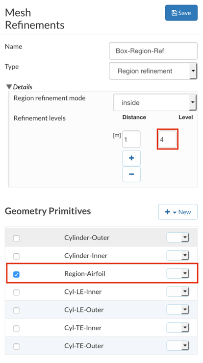
Figure 21: Shows where Level is defined and the primitive assigned to this region refinement.
To define the rest of the region refinements, use the same technique as above but with the settings and assignments indicated in the table below.
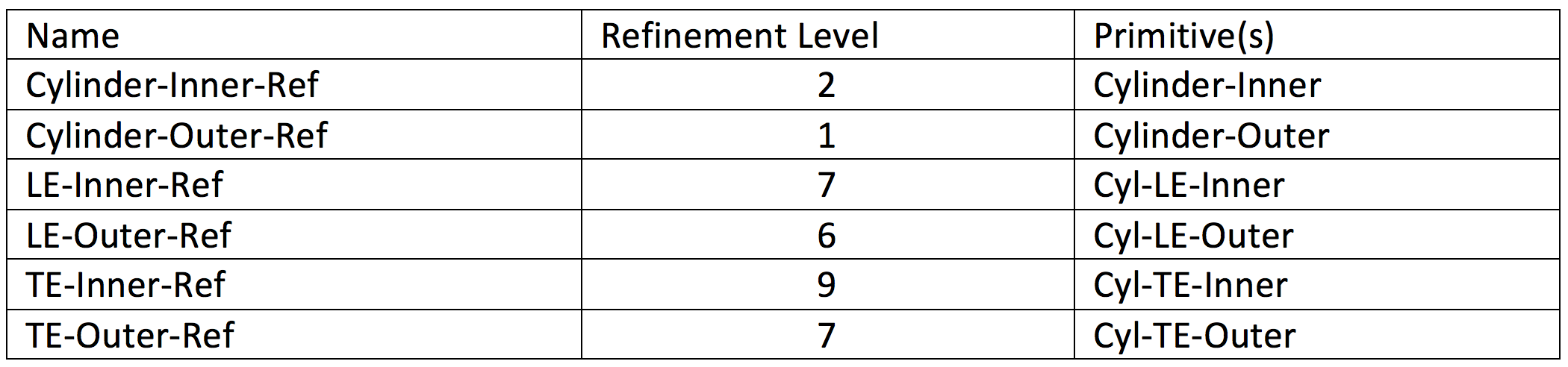
Figure 22: Table shows settings for Name, Level and Assignment for Region Refinements.
After these refinements are defined please check them off against the node tree list below before proceeding.
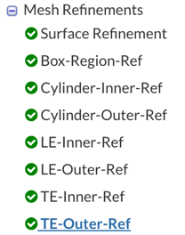
Figure 23: Shows created refinements to be checked off against own setup.
Duplicate the mesh by right-clicking the mesh in the node tree and selecting Duplicate, being very careful not to accidentally select Delete.
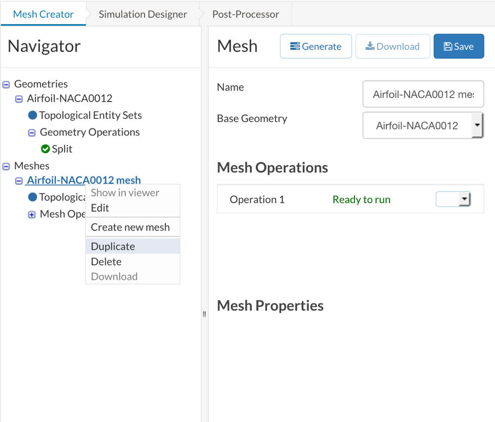
Figure 24: Duplicate mesh to make an exact copy of the mesh setup as a basis for our next mesh.
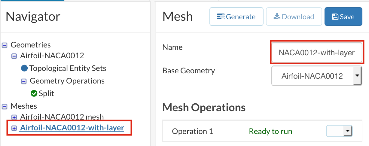
Figure 25: Renaming the mesh to Airfoil-NACA0012-with-layer.
Whilst we do some modifications to the setup of the new mesh, start running the original mesh by either selecting it and pressing Generate or select the Operation within the mesh and pressing run.
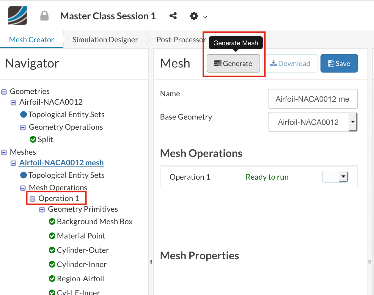
Figure 26: Both methods of starting the mesh operation.
Once the new mesh has started, return to the new mesh Airfoil-NACA012-with-layer and add an additional refinement, Name as Surface Layers and Type as Inflate Boundary Layer this refinement creates thin layer cells at surfaces boundary so that the boundary layer can be better resolved. For this mesh, we simply want to be able to see the difference between not having layers and results with a single layer. Later we shall correctly define the boundary layer looking at the Y+ value. Use the following settings.

Figure 27: Adding Surface Layers
Select the airfoil surface and to be the surface with layers and commit the settings by selecting save. As done before, start this new mesh by using either generate or run. Once both meshes have completed compare the two and observe the difference in near-surface meshing as highlighted below.
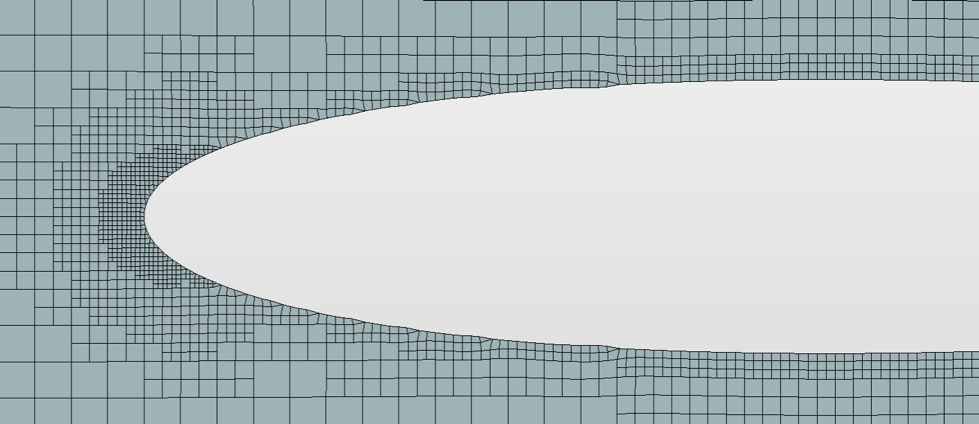
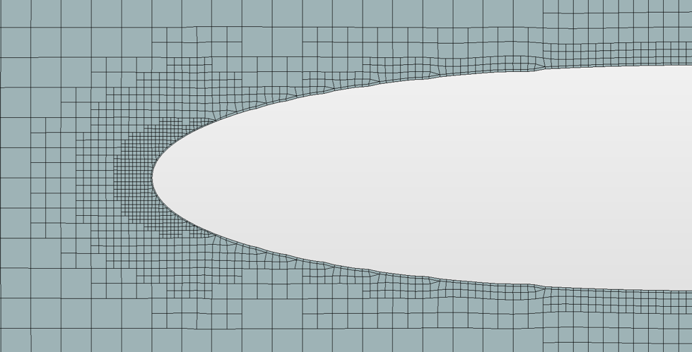
Figure 28: Comparison between mesh with and without a layer.
Now we have two meshes to compare we will proceed with simulation setup in order to observe the difference between results.
Simulation Setup
Navigate to the Simulation Designer tab in the SimScale Workbench and click on +New to create a new simulation setup.
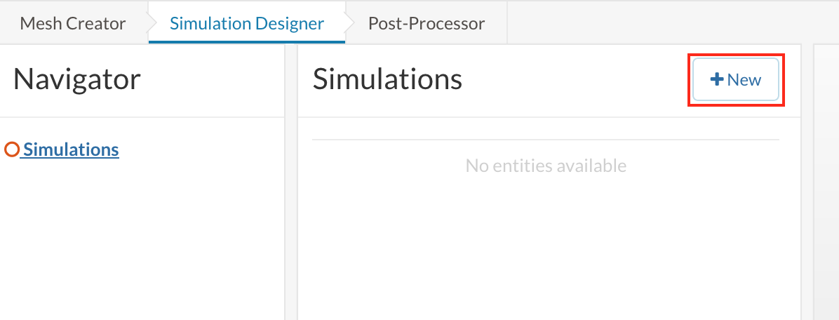
Figure 29: Creating new simulation.
A window will pop up, asking you to select the type of analysis. Click on Incompressible in the category Fluid Dynamics. Click Save to close the pop-up.
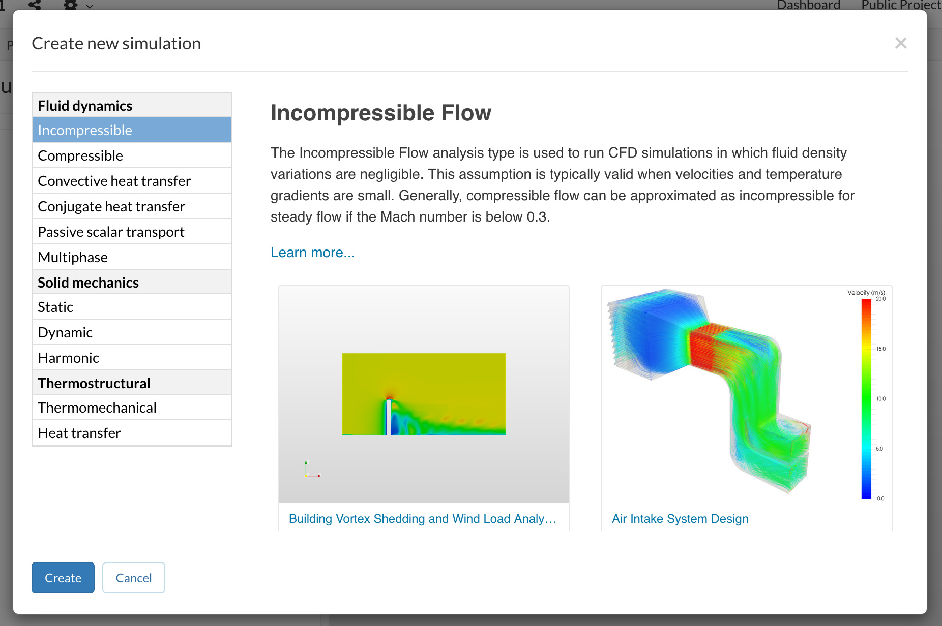
Figure 30: Choosing the type of analysis
Ensure that the settings are steady state and that the turbulence model is K-Omega SST.
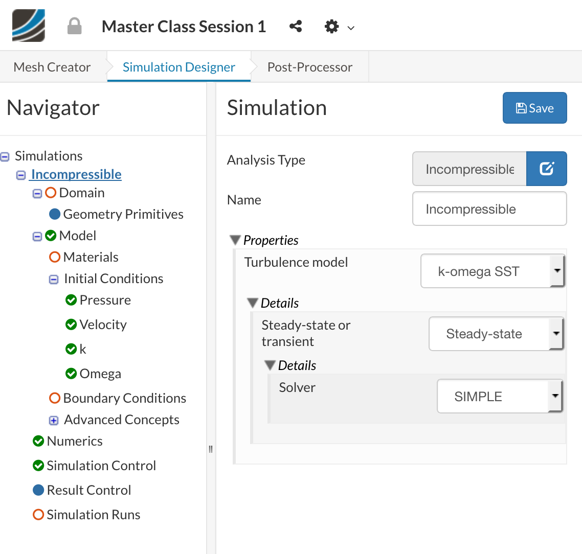
Figure 31: Incompressible settings.
Next, select the mesh that you first created, Airfoil-NACA0012 mesh.

Figure 32: Choosing the required mesh
Click Save to store your progress.
Materials
Next, we need to define a material and assign it to the mesh region. Select Materials and import from material library, choose Air and at the bottom save.
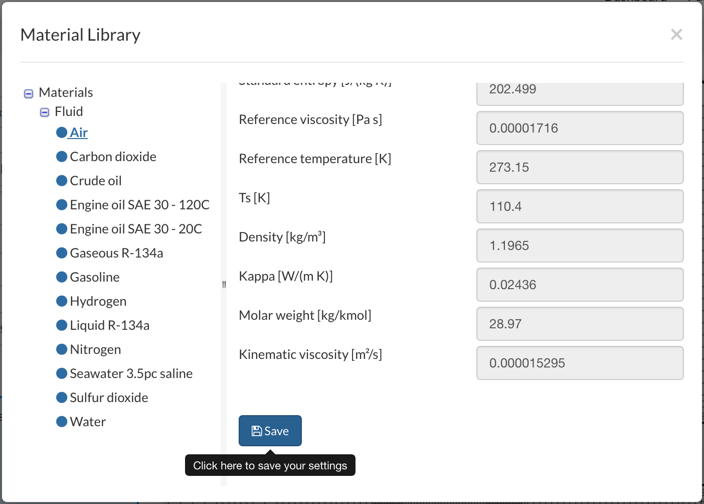
Figure 33: Importing Air as a material.
Assign it graphically to the mesh region in the viewer, and save to commit the changes.
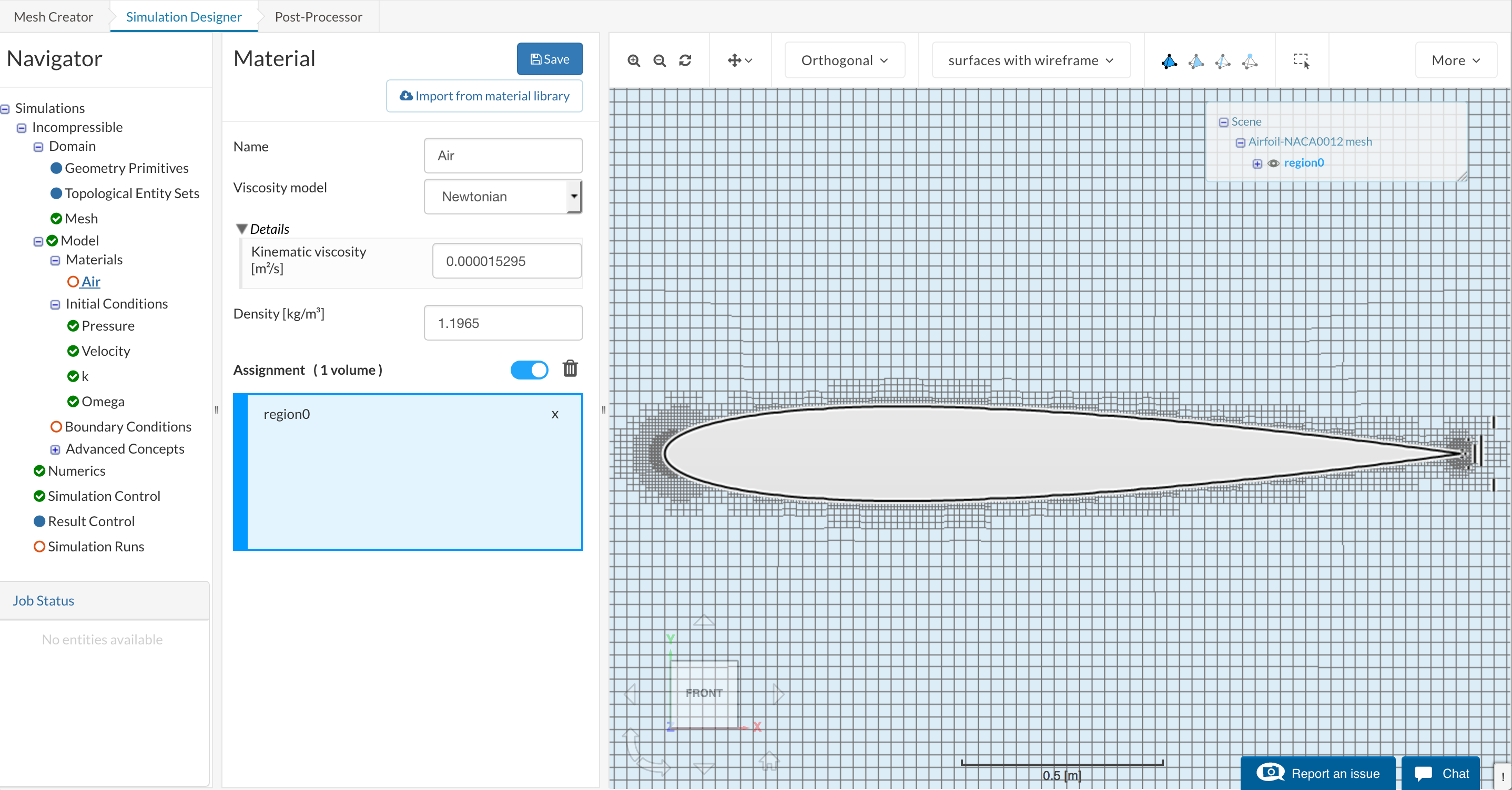
Figure 34: Assigning Air to the fluid domain.
Initial Conditions
The first part of our setup requires us to apply and approximate certain conditions to the domain at time 0. These initial conditions in steady state can heavily affect stability and time to convergence, so it is worth spending some time correctly defining these conditions.
Set the Pressure to a uniform 119650Pa
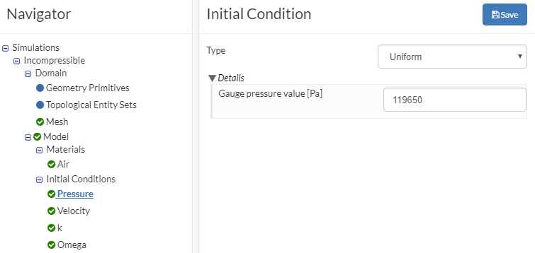
Figure 35: Set initial Pressure.
Set the Velocity to a 9.8281m/s in the x-direction and 1.7365m/s in the z-direction. This creates an angle of attack of about 10 degrees.
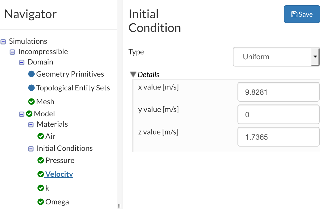
Figure 36: Set initial Velocity.
Set the Turbulent Kinetic energy (k) to 0.0006 m^2/s^2
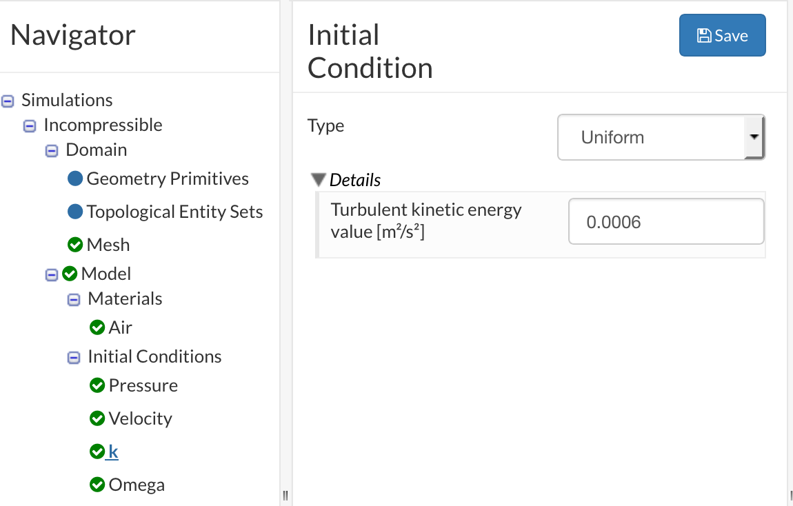
Figure 37: Set initial Turbulent Kinetic energy (k).
Set the Specific Dissipation Rate (Omega) to 4.472 1/s:
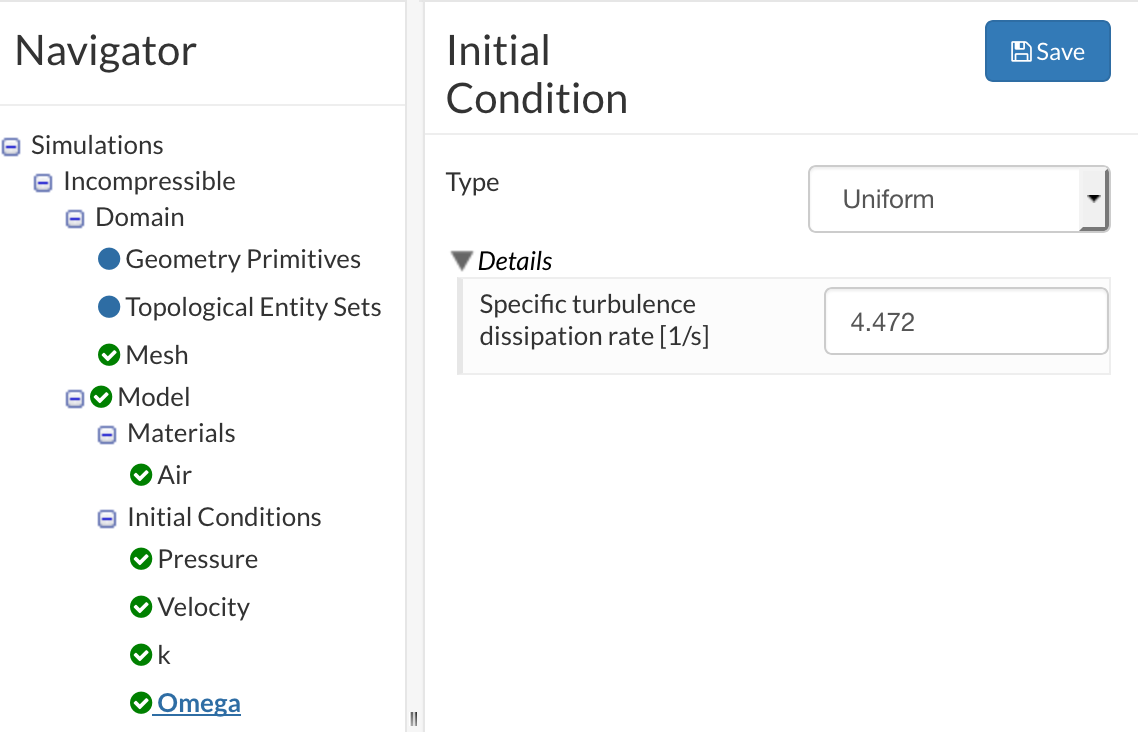
Figure 38: Set initial Specific Dissipation Rate (Omega).
This concludes the initial conditions required for an incompressible flow problem.
Boundary Conditions
Boundary conditions define how the fluid moves into and out of the system, and how it interacts with any object within the domain or at its boundaries. A lot of problems can occur if incorrect or poorly defined boundaries are used. The following boundary condition setup allows for an angle of attack to be defined and altered without the need of geometry or mesh changes.
Create a new boundary condition by selecting Boundary Conditions and selecting +New, alternatively, the Boundary Conditions node in the node tree can be right clicked to Add Boundary Condition.
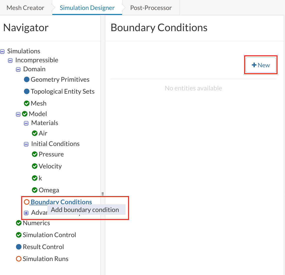
Figure 39: Add a new Boundary Condition.
Change the Type to Symmetry and rename the condition Symmetry Walls. Finally, graphically select the two side boundary walls and commit changes using Save.
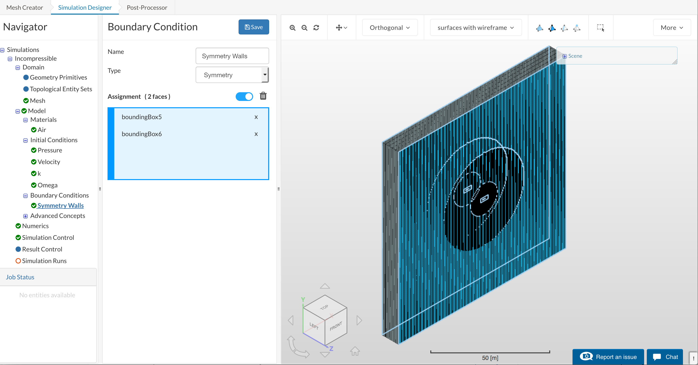
Figure 40: Symmetry settings, with visible assignments.
Create another Boundary Condition, this time change its type to Custom and change its name to Far-Field. This boundary is for the inlet-outlet condition, set it up with the following settings and assign it graphically to the four edges as indicated.
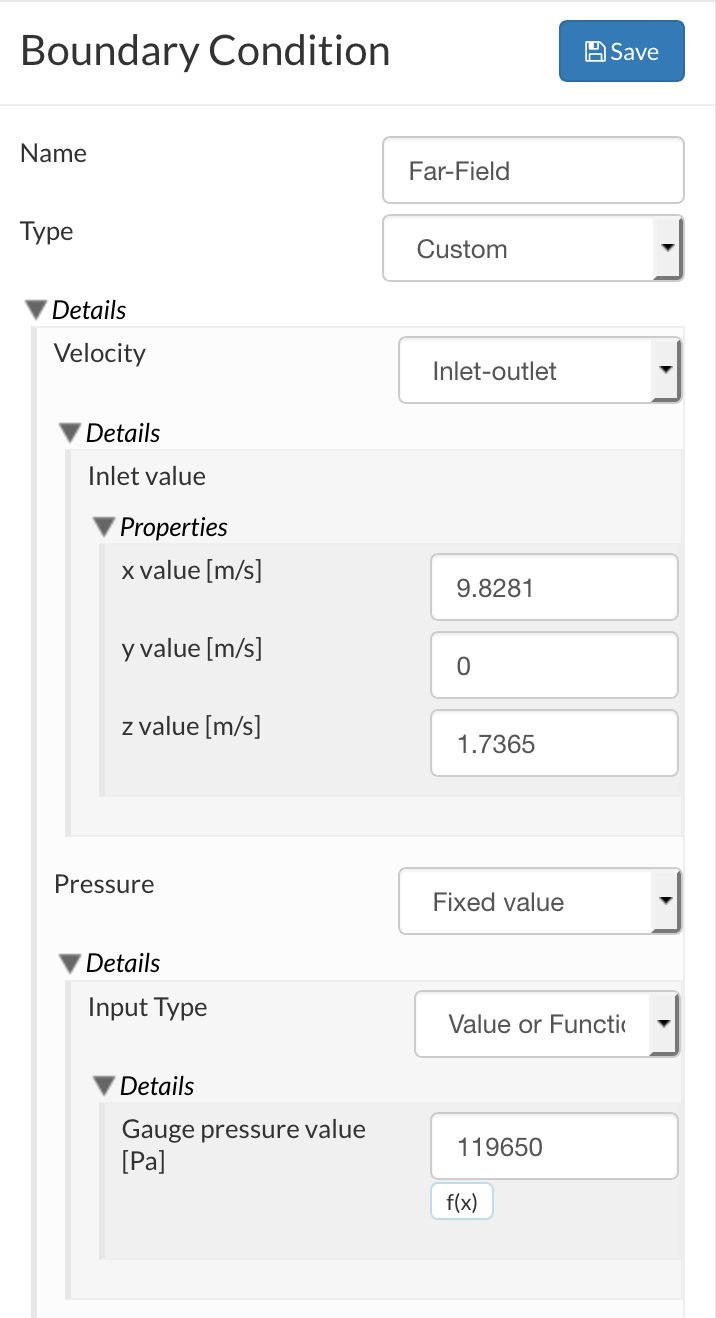
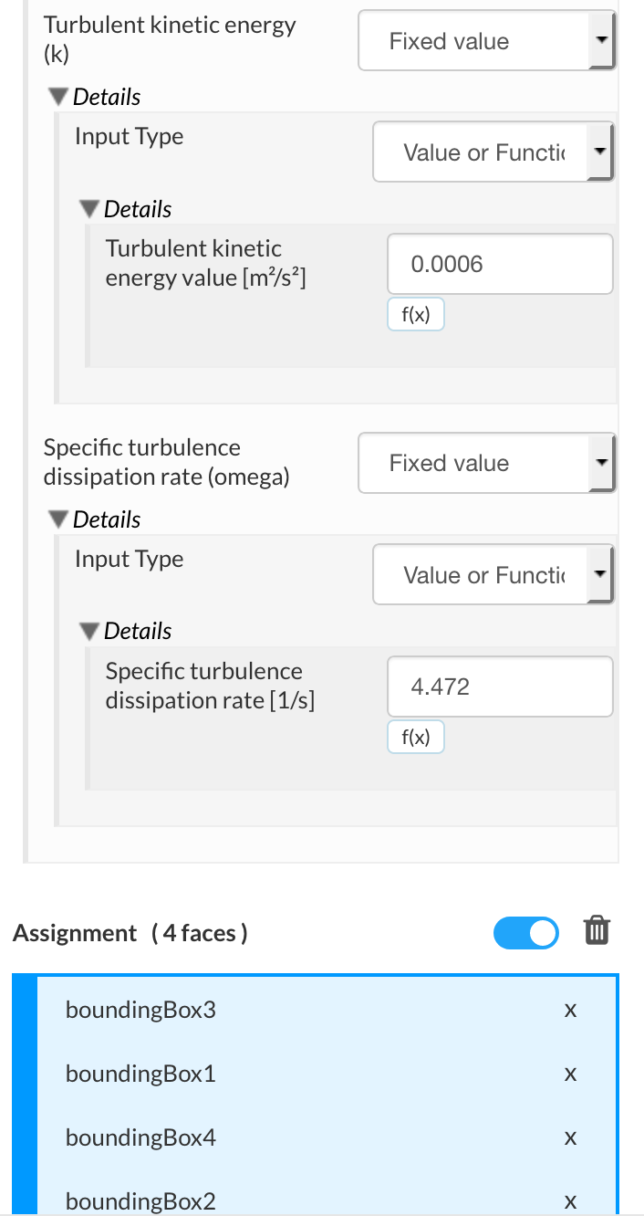
Figure 41: Inlet-outlet condition settings, Velocity and Pressure on the left and Turbulence and Assignments on the right.
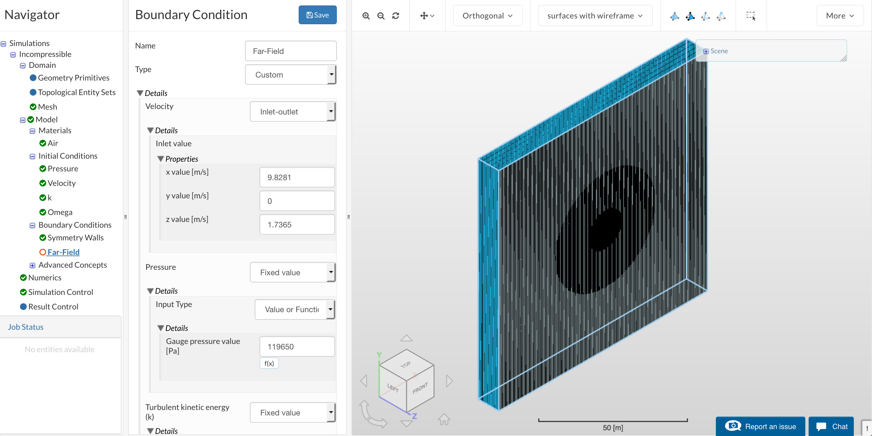
Figure 42: Inlet-outlet condition visible assignment.
For the last boundary condition, create a new condition as before and alter Type to Wall and change the name to Airfoil. Ensure that No-Slip is selected and assign the airfoil wall to the condition this can be done by selecting the airfoil directly or selecting the bounding walls and Invert visible assignment by right-clicking in the viewer:
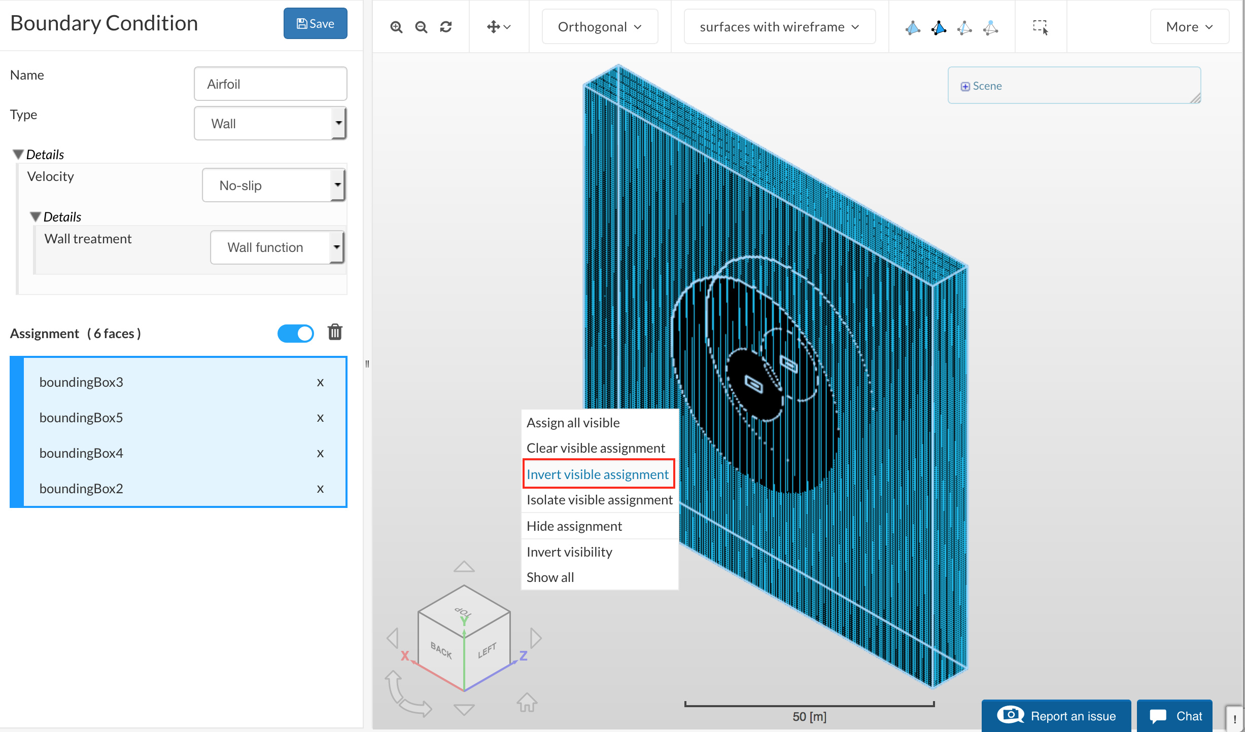
Figure 43: Invert assignment to select airfoil.
Now that the boundary conditions have been defined, we will move onto the final stage of setting up the simulation by altering Numerics, Simulation Control and Result Control.
Numerics
Under Numerics in the node tree, change the under-relaxation factors and absolute tolerance to match those depicted below.
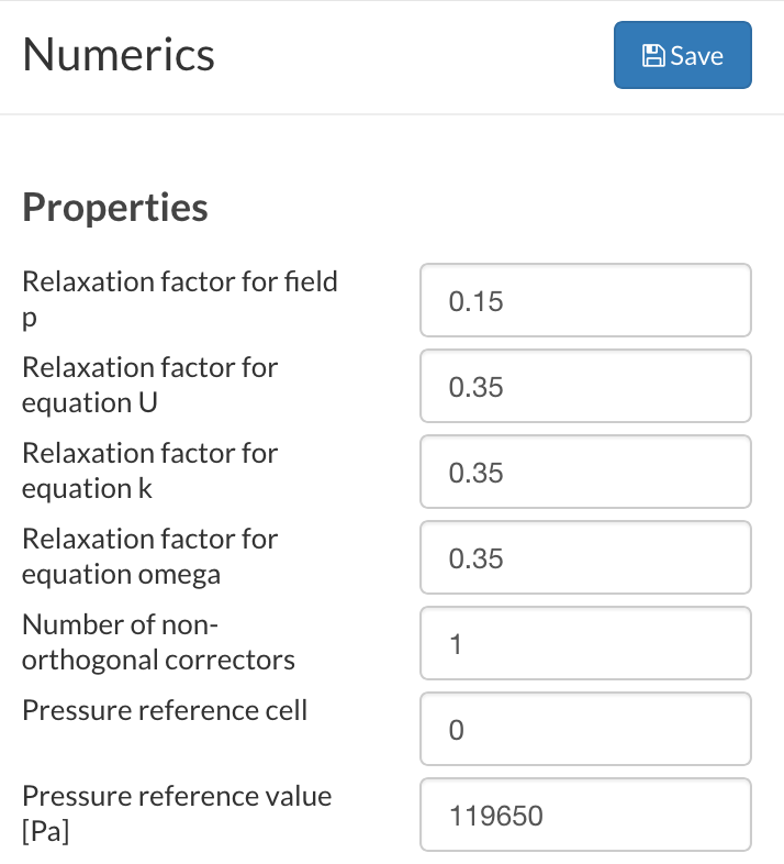
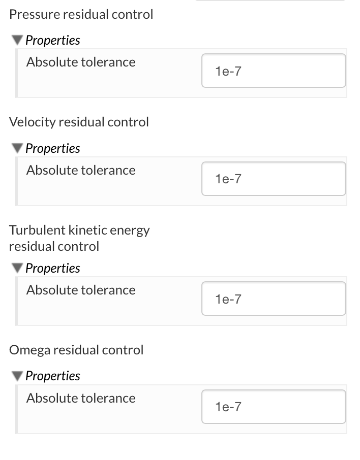
Figure 43: Numerics settings for relaxation factors and absolute tolerance.
Relaxation factors help stabilize a solution that might otherwise not converge, whilst absolute tolerance sets the termination criteria to be met, so in this case, if the residuals fall below 1e-7 for all variables then the solver will terminate without performing any further iterations.
In the same Numerics Tab, some additional changes need to be made to the solvers, this includes changing the pressure solvers tolerances and pre-sweeps, altering the velocity and both turbulence solvers to smooth solvers and adjusting their tolerances. Make the changes as depicted below.
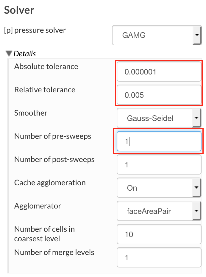
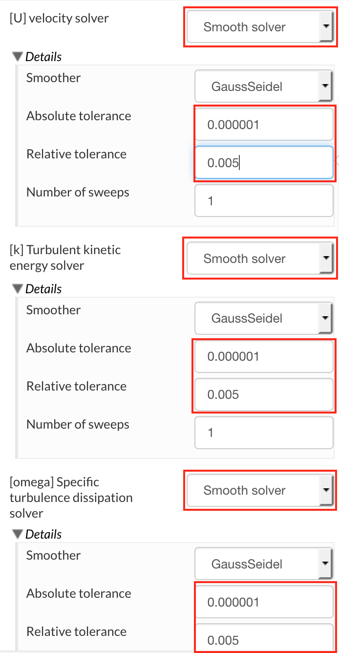
Figure 45: Numerics settings individual solvers.
Simulation Control
In the simulation control panel, a few alterations need to be made. End time value (s) needs to be increased as convergence might take longer than 1000 iterations and the number of computing cores needs to be increased to ensure that enough processing power and ram is allocated for the larger mesh. Finally, Maximum runtime needs to increase, this ensures that real-time restrictions will not end the simulation, but at the same time if for some reason it goes on for an exceptionally long time then the simulation will stop. Please make the changes as depicted below and remember to commit the changes by saving.
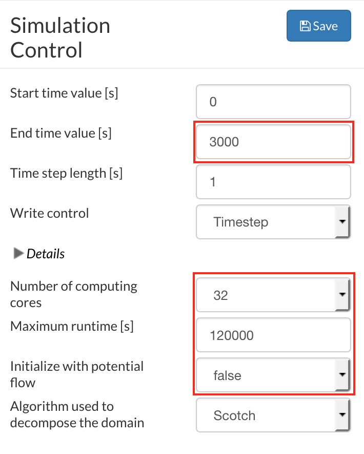
Figure 46: Simulation control Setting.
Result Control
In the Result control panel, there are options to add additional fields and plots. Because we are interested in the boundary layer and its effects, we will need to create result control items for forces and moments acting on the airfoil and Y+ values.
Start by adding a new result control item under Forces and Moments by clicking +New.
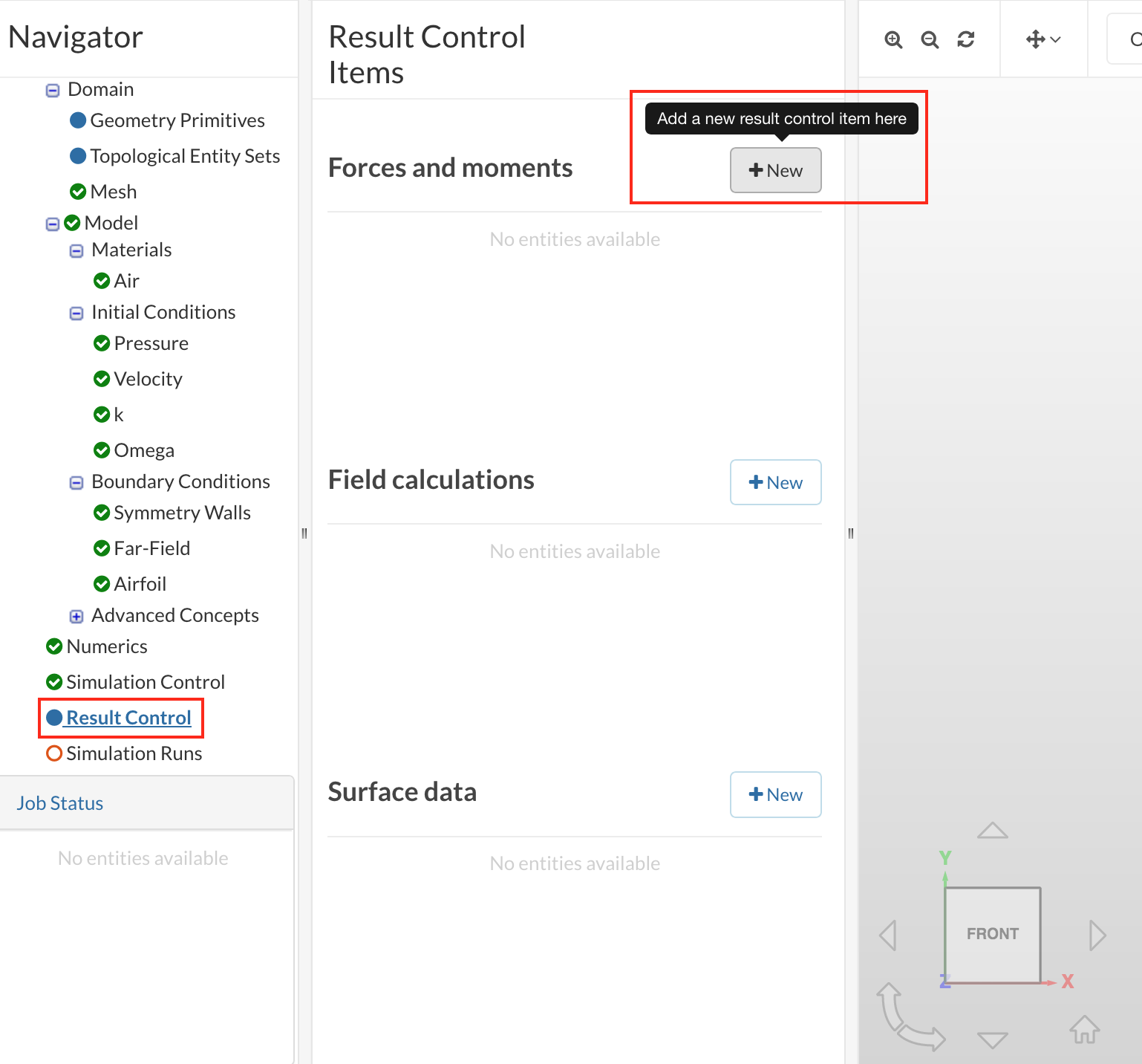
Figure 47: Result Control panel, with annotation for Forces and Moments.
Once it is added rename it Forces, change the write interval to 10 and nominate the airfoil surface for the assignment. The centre of rotation can be left as [0, 0, 0] because we are mainly interested in lift and drag and not in the moments acting around a point.
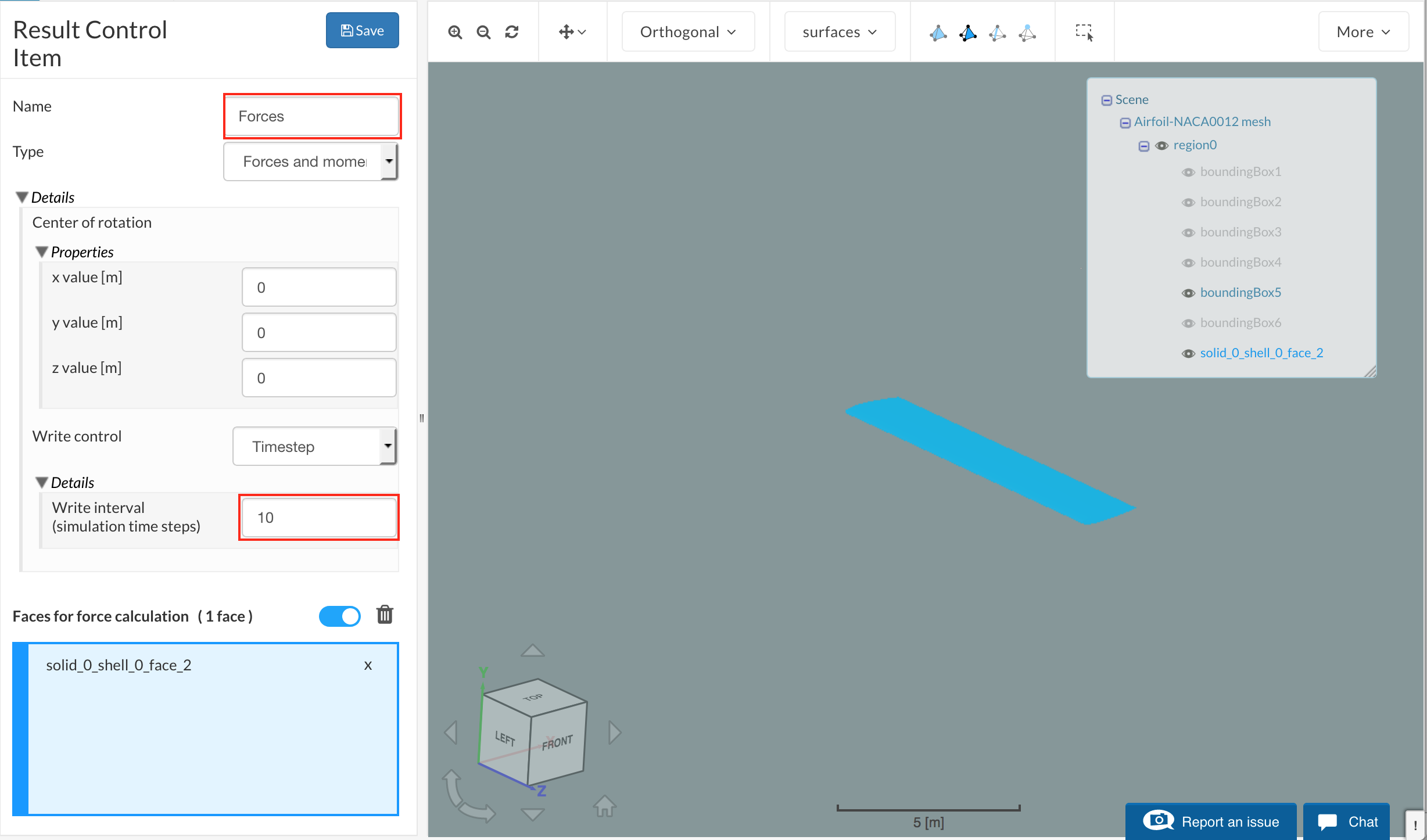
Figure 47: Forces result control with settings.
The next result control will look at the Y+ value at the nearest cell to the surface. This helps us to determine if the wall cells have been under or over resolved for the particular wall model. Start by adding a field calculation in the Result control panel by selecting +New next to the Field Calculations.
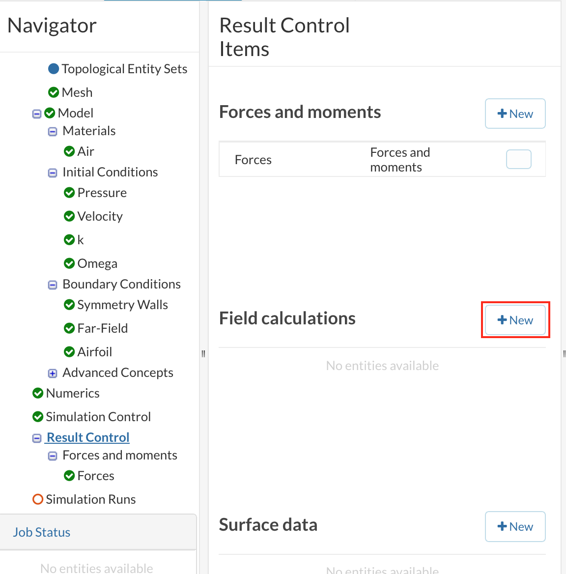
Figure 48: Adding a Field Calculation, Result Control Item.
Apply the following settings.
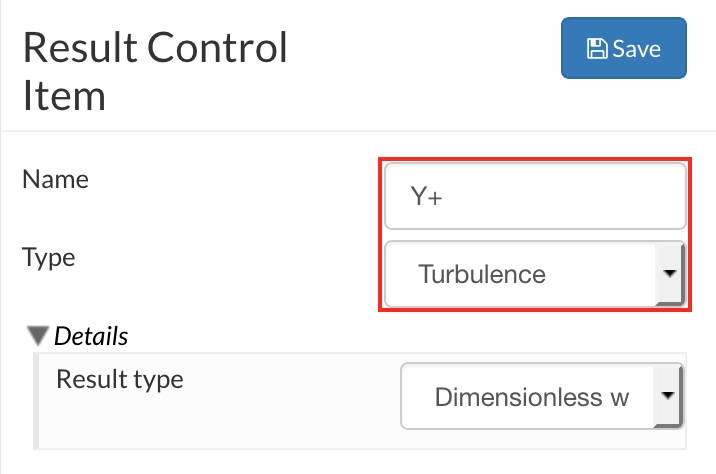
Figure 49: Settings for Y+, Result Control Item.
Simulation Runs
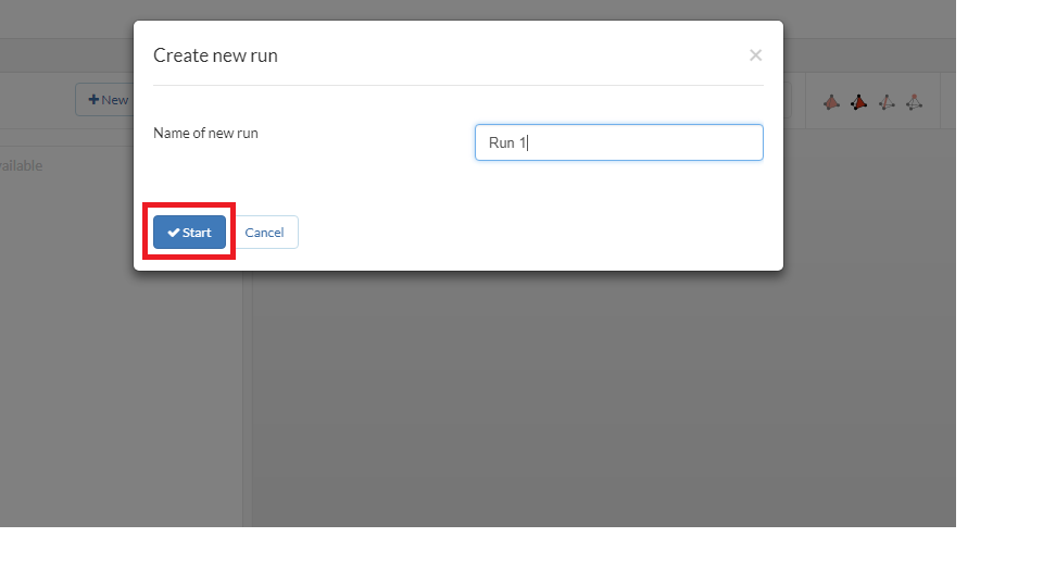
Finally, navigate to the simulation runs panel and check the setup, if no errors or warnings are present, click +New to make a new run and click Start to run the simulation.
Creating Further Simulations
To save time in simulation setup, we can duplicate the current simulation setup and assign a different mesh to it. Then the only setup required is to reassign anything that required an assignment. To do this start by selecting the original simulation in the node tree, right click and select duplicate (be really careful not to delete here).
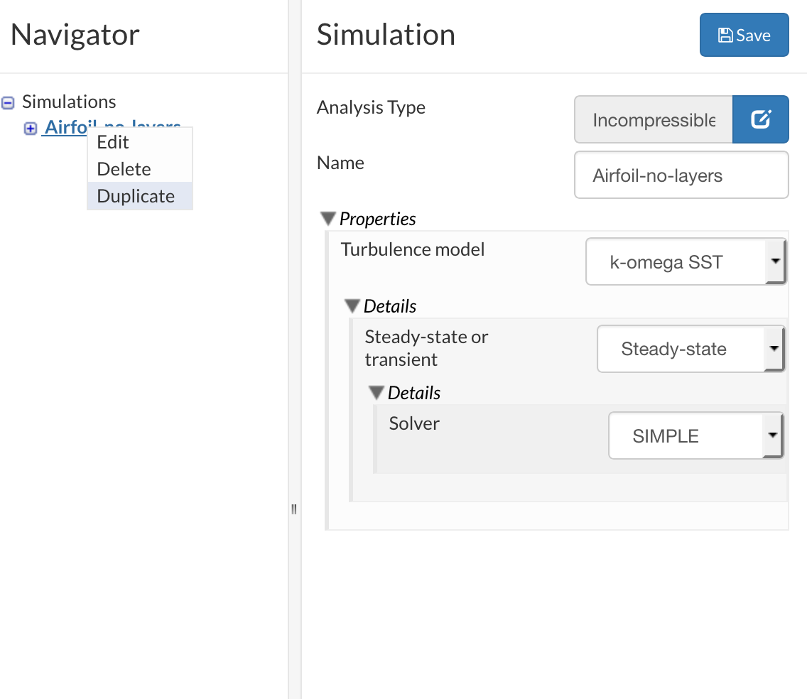
Figure 50: Duplicate simulation to run it with another mesh.
Once this has been duplicated select the copy and rename it to Airfoil-1-layer.
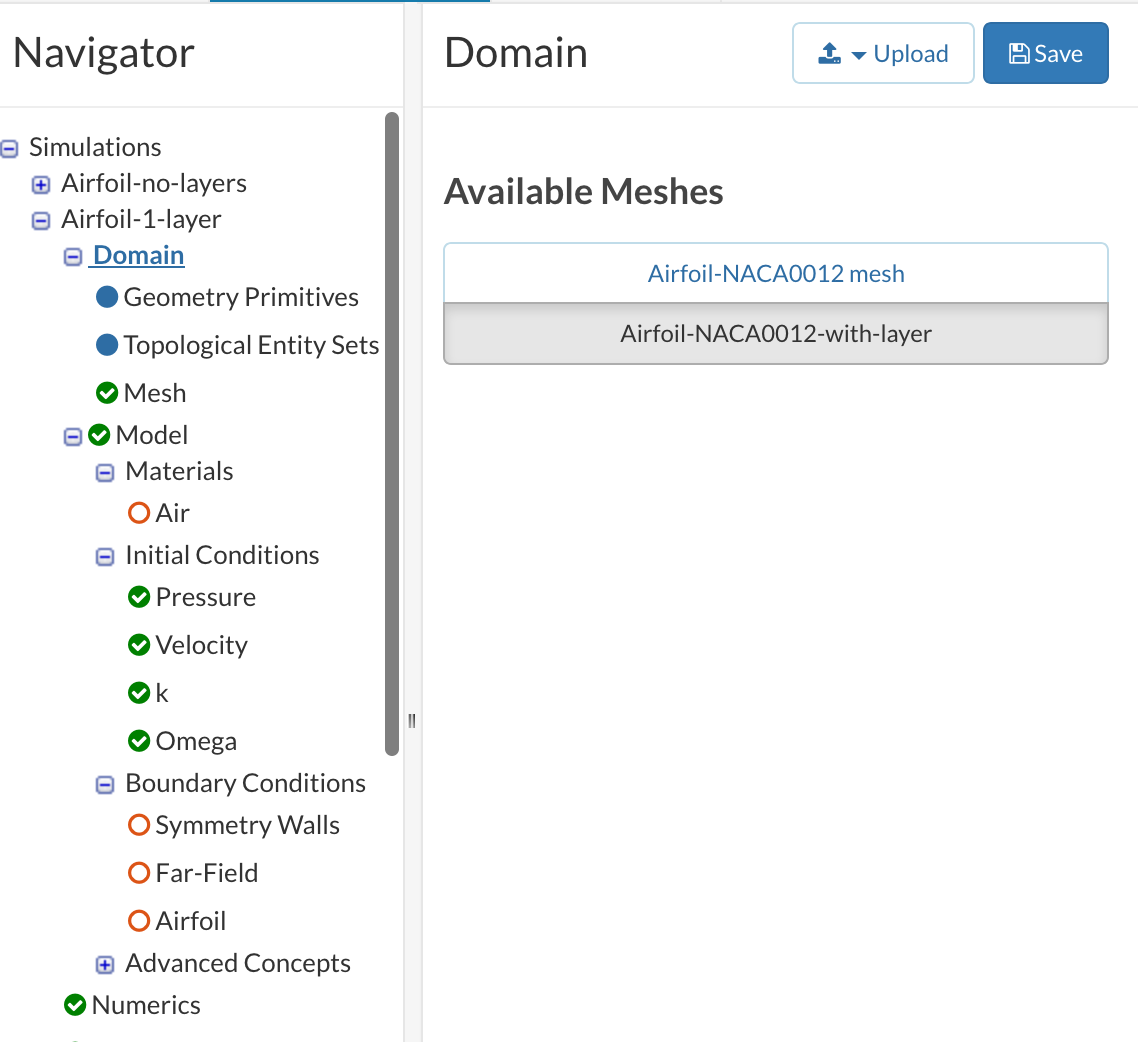
Figure 51: Alter the mesh in the new simulation.
Work through the node tree reallocating assignments to; Materials, Boundary Conditions and Result Control Items. Once this has been completed, check the simulation and create a run.
When the simulations finish, the results can be post-processed online to visualise the results.
Post-Processing
To observe the difference in velocity profiles it will be necessary to take the raw data and filter it to observe results more relevant to us. To do this we shall firstly look at and compare the velocity field on a plane to ensure that results are smooth, and then we shall observe Y+ values to determine if the mesh models the boundary layer correctly.
Velocity Profile
Firstly, move to the Post-Processing Tab and select the simulation results for the simulation Airfoil no layers.
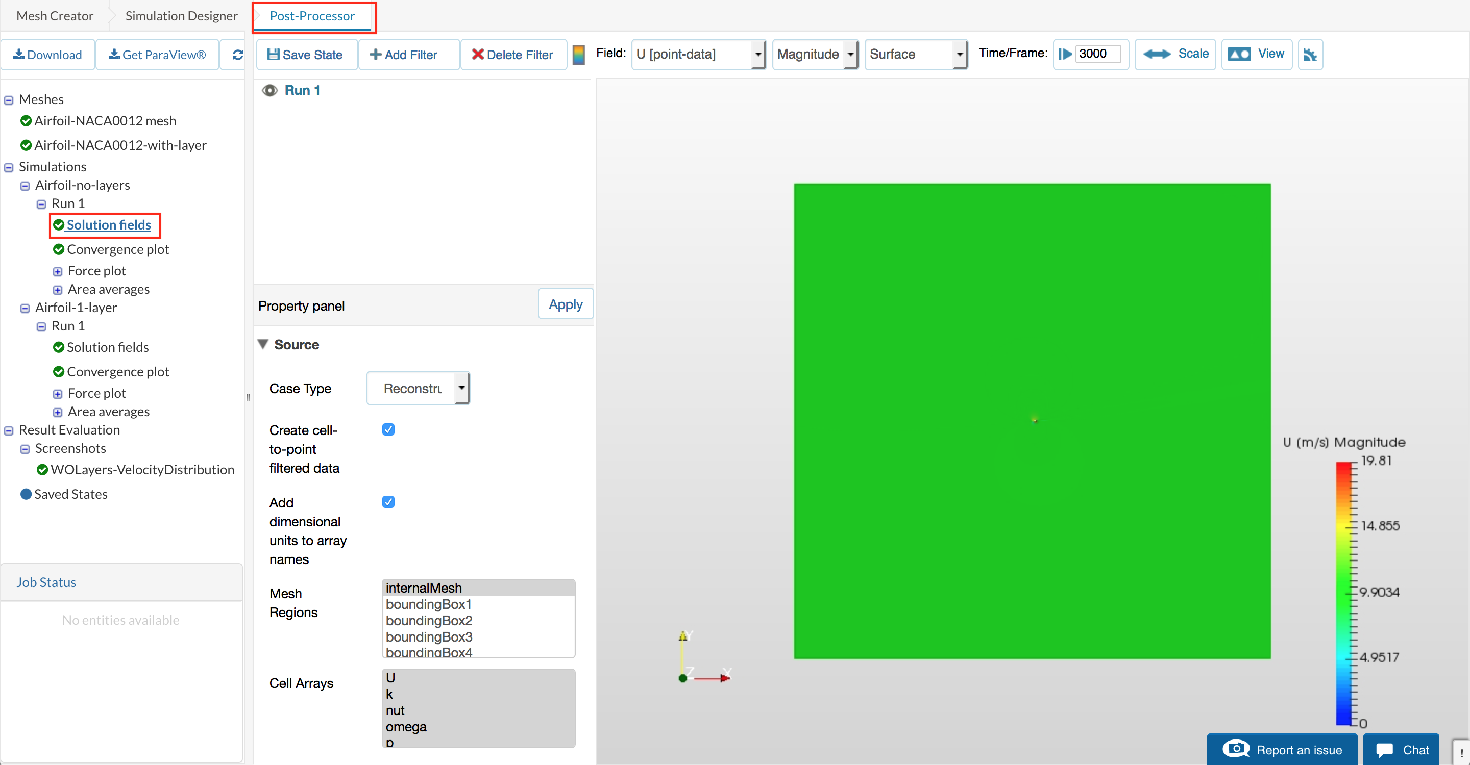
Figure 52: Change to Post-Processing Tab and load Solution Fields for Airfoil-no-layers.
Now add a filter by selecting the +Add Filter button and then select Slice from the drop-down menu.
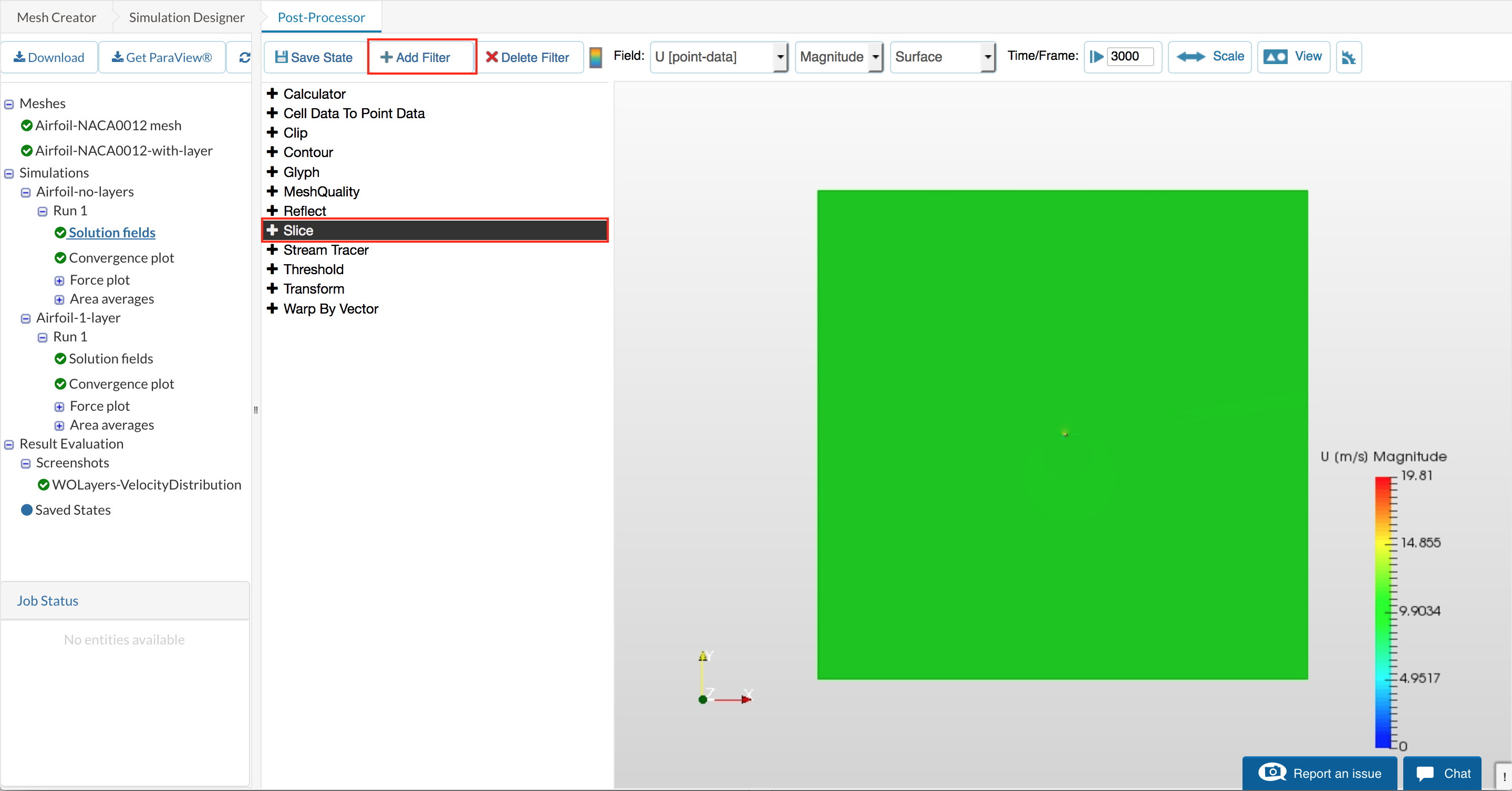
Figure 53: Create a new slice filter, selecting +Add Filter then Slice.
Select the slice and alter the slice settings in the panel so that the filter is in the plane of the flow (XY Plane), this can be done by altering normal to the z plane by giving the normal vector (0, 0, 1). Whilst in the slice panel is open deselect Show Plane.
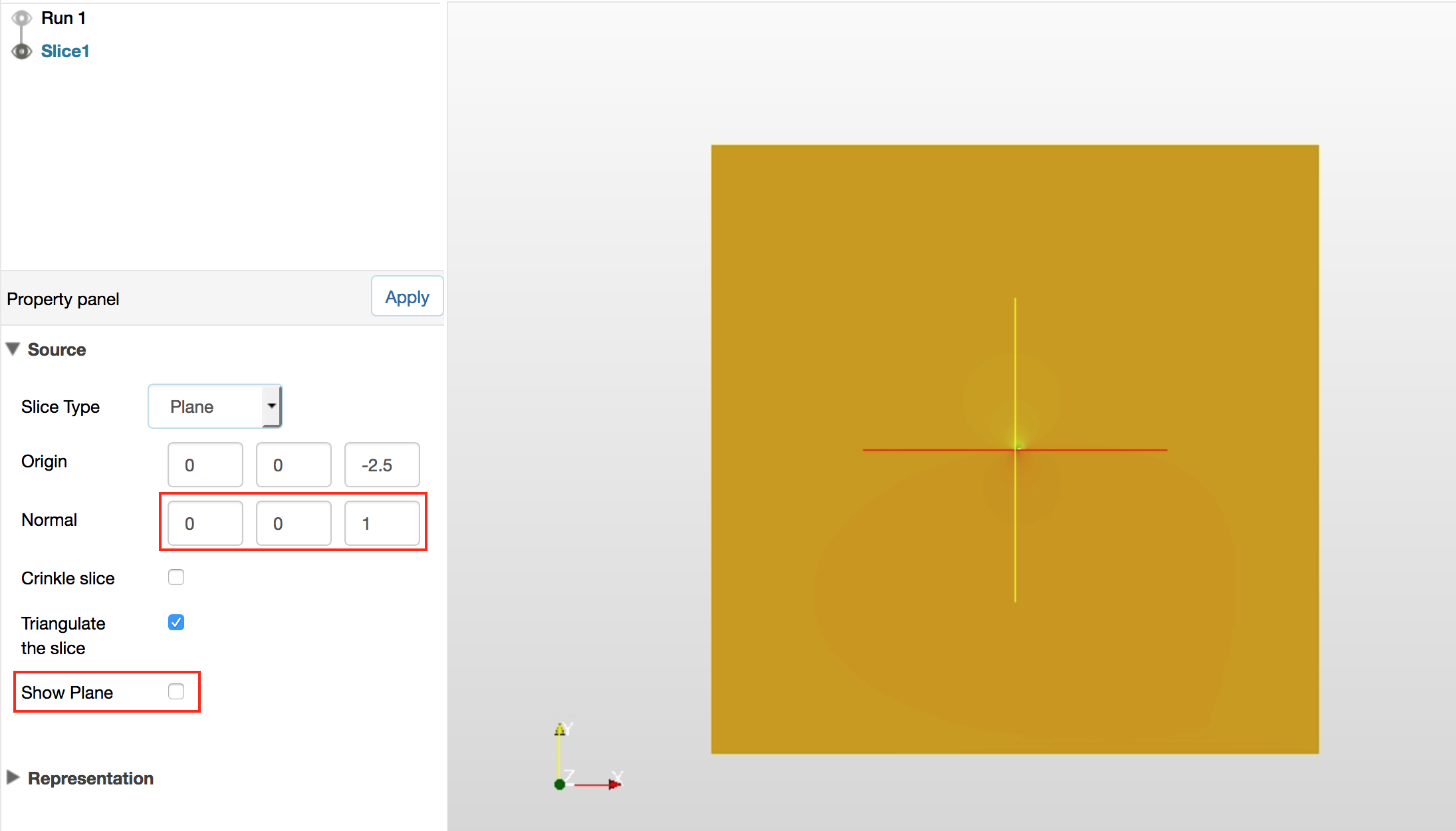
Figure 54: Alter the Normal vector, and deselect the Show Plane option.
Finally, alter the representation field to Velocity, U (point-data) and hide the centre of rotation crosshairs by navigating to the menu button View, and selecting the Toggle visibility centre of rotation button on the left as depicted below.
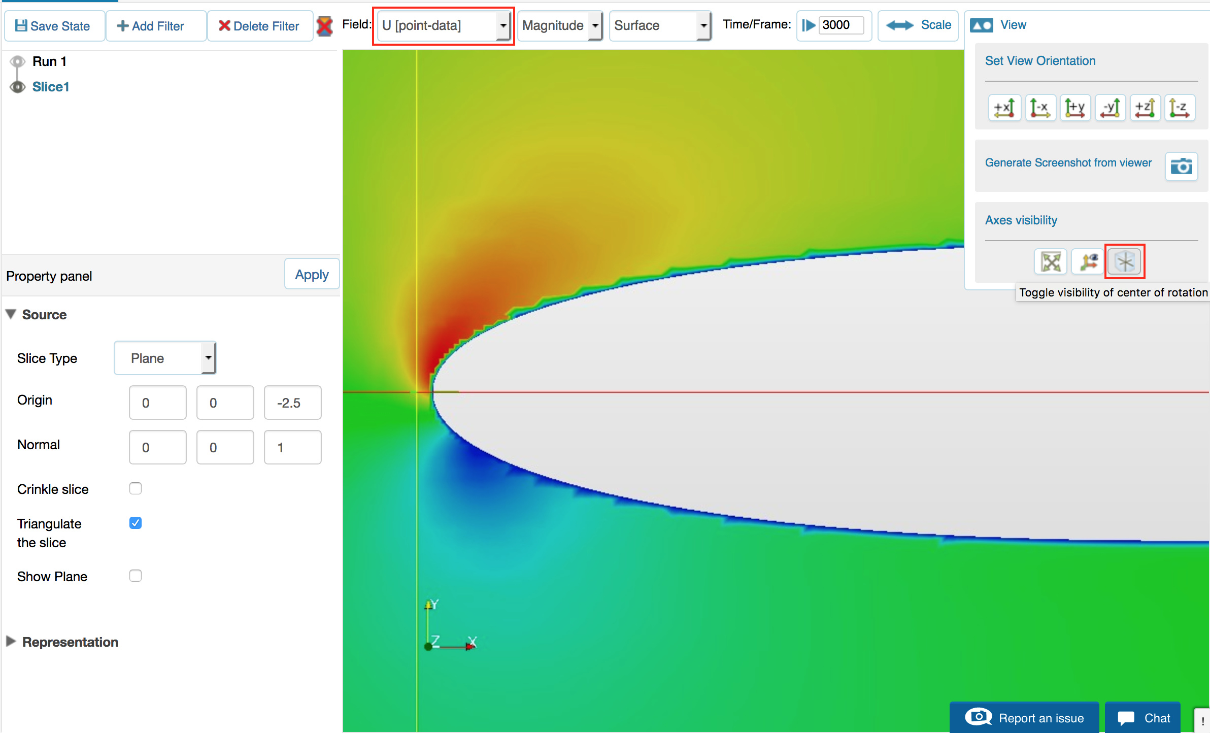
Figure 55: Change field to U (point-data), and remove center of rotation lines.
Add the legend so that velocity values are easily identifiable from the colour map, this is available just before the field display option in the top bar.
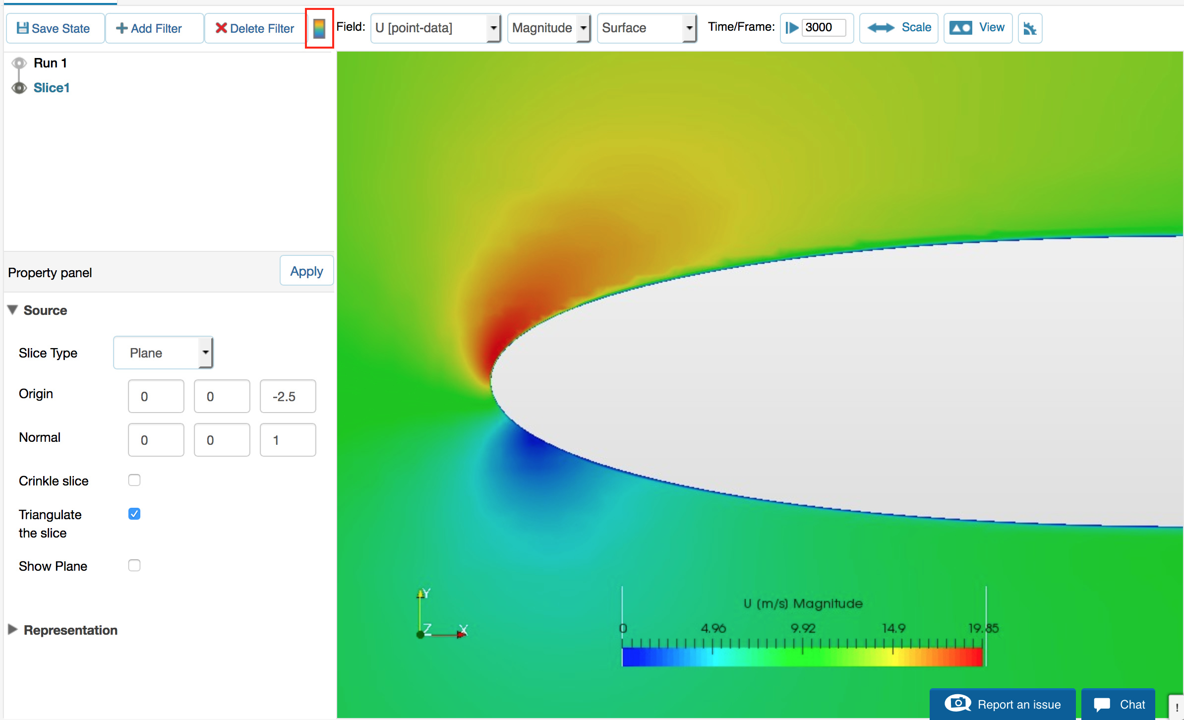
Figure 56: Add legend by toggling the legend display button.
Create a screenshot of the Post-Processing state by navigating once again to the view option in the menu, and select the generate screenshot button.
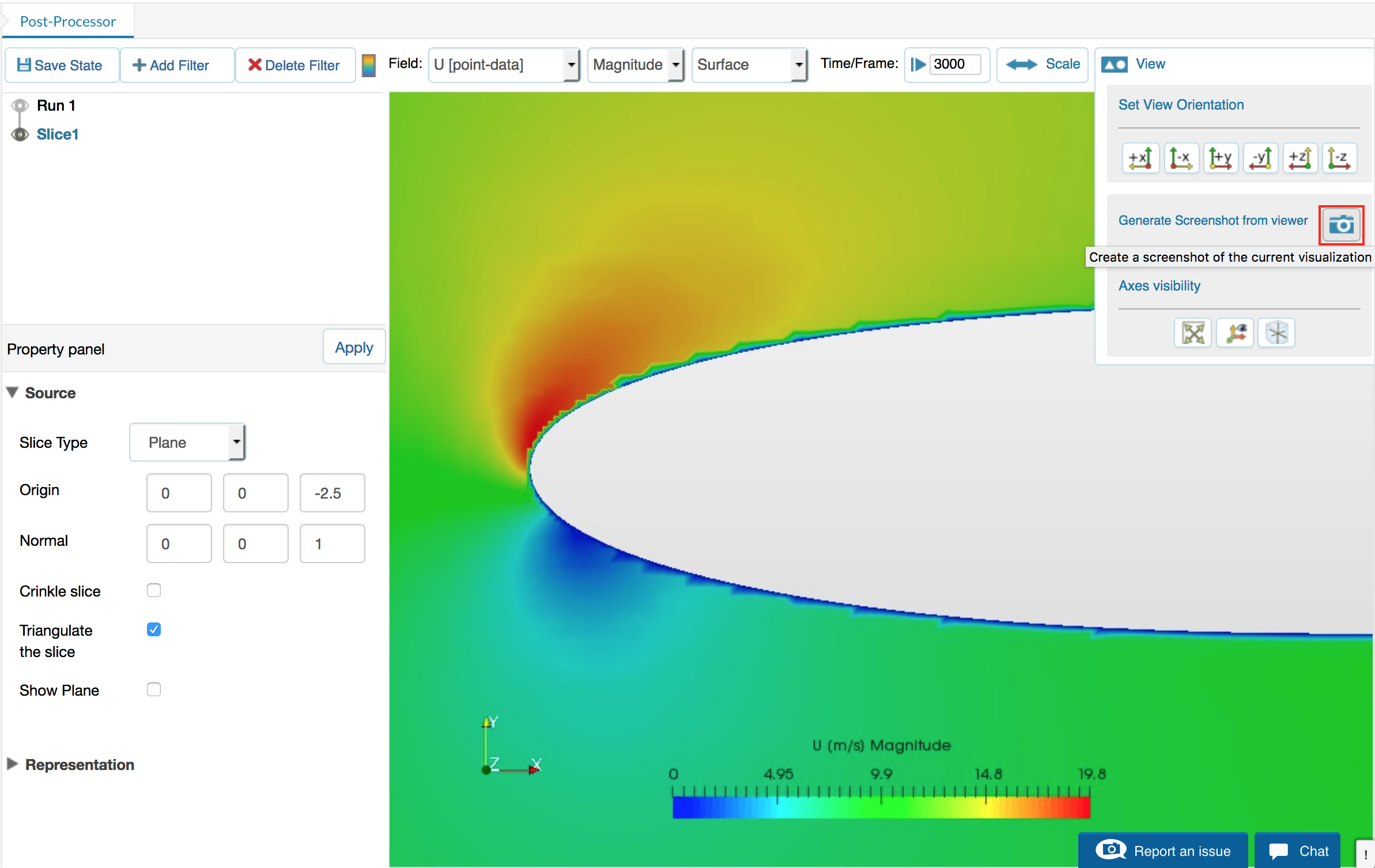
Figure 57: Generate a screenshot.
Rename the screenshot to describe the image, for example, NoLayers-VelocityDistribution. This can be found under screenshots, then change the name in the screenshot panel.
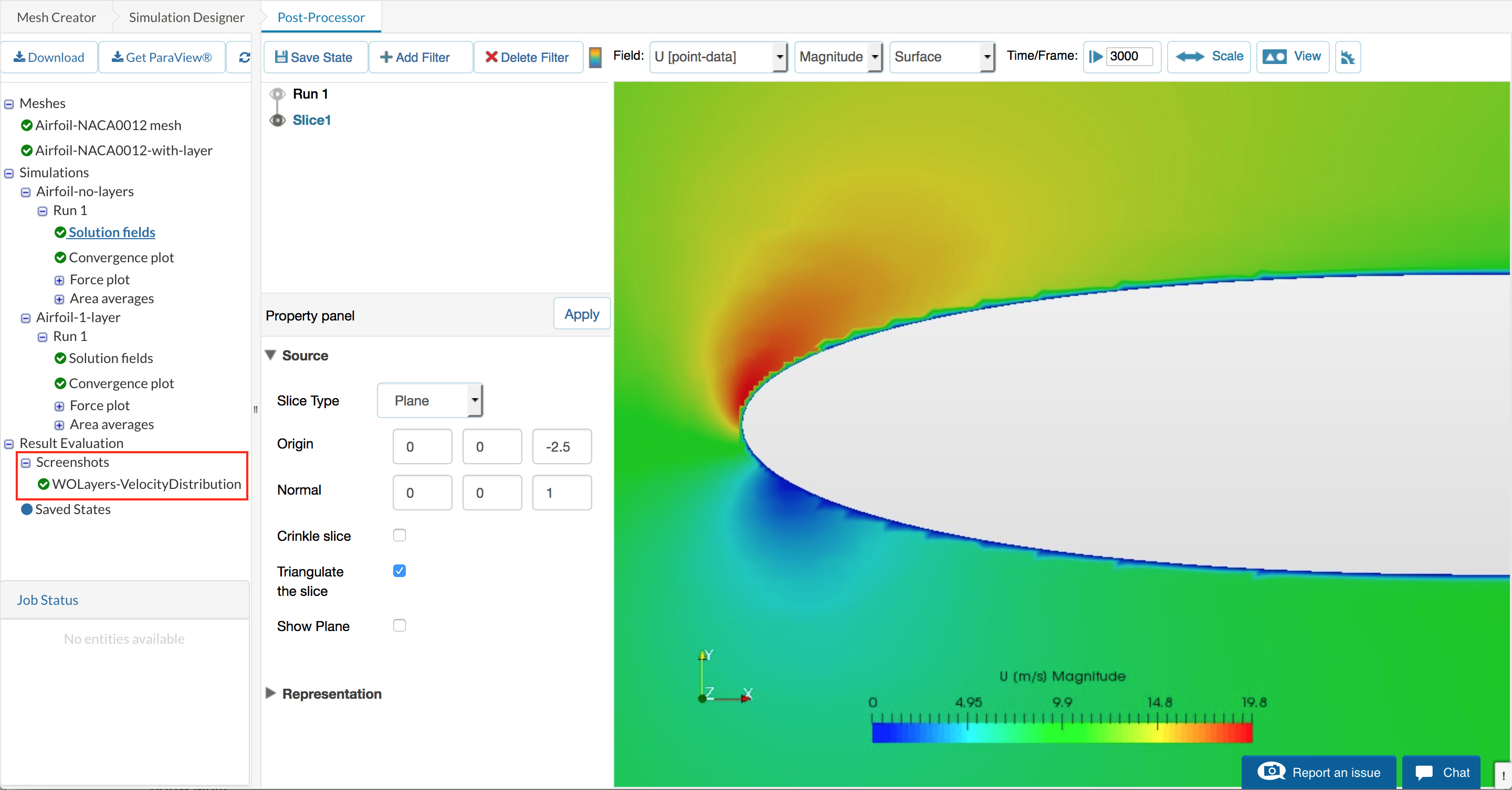
Figure 58: Select the screenshot under Screenshots.
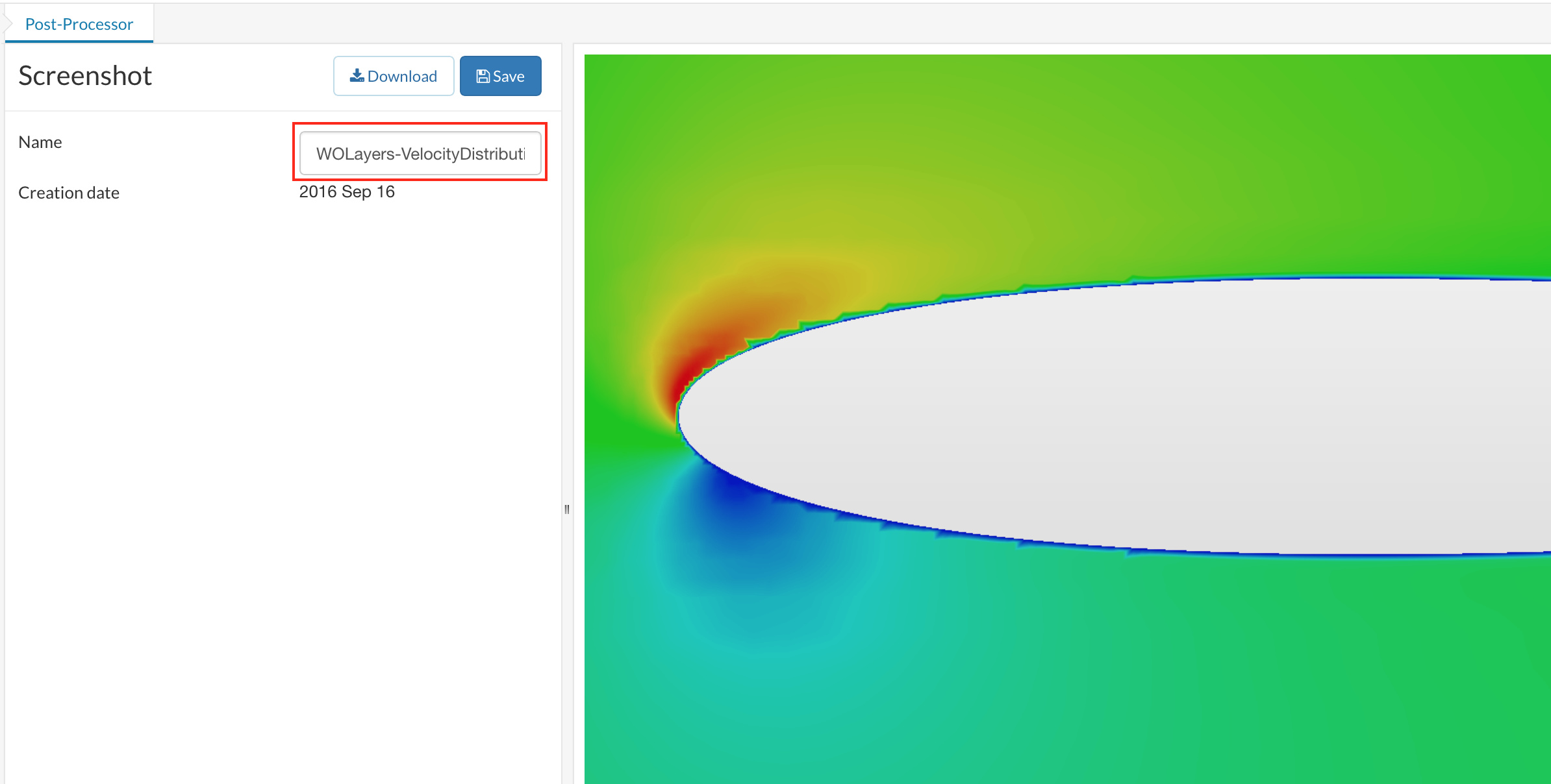
Figure 59: Change the name to describe the image.
Do the same again for Airfoil-1-layer and save the screenshot for comparison.
Aerofoil Y+
It is also important to analyse the Y+ value and to determine how much it affects results. To do this we can look at Y+ values on the surface of the foil and compare those values to our target Y+ value.
To do this, start in the same way as before and bring in the solution fields for no the simulation with no layers.
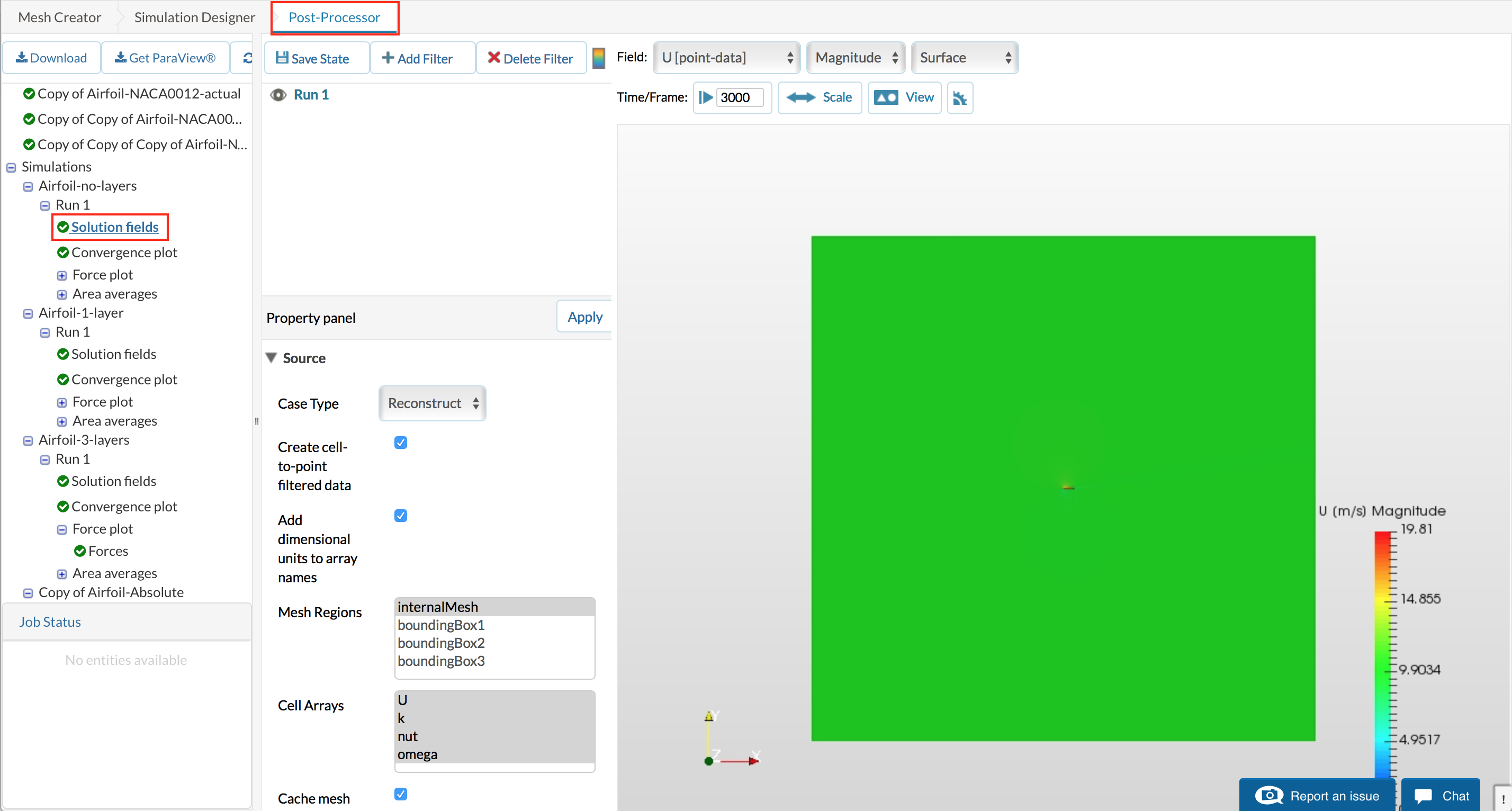
Figure 60: Open the solution fields into the viewer.
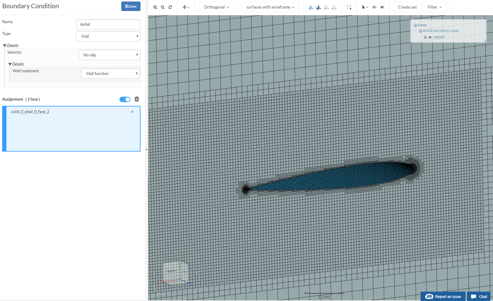
Now we can change the mesh regions to show only the airfoil surface. This is done by navigating to the Mesh regions in the panel and selecting only solid_0_shell_0_face_2 and apply.
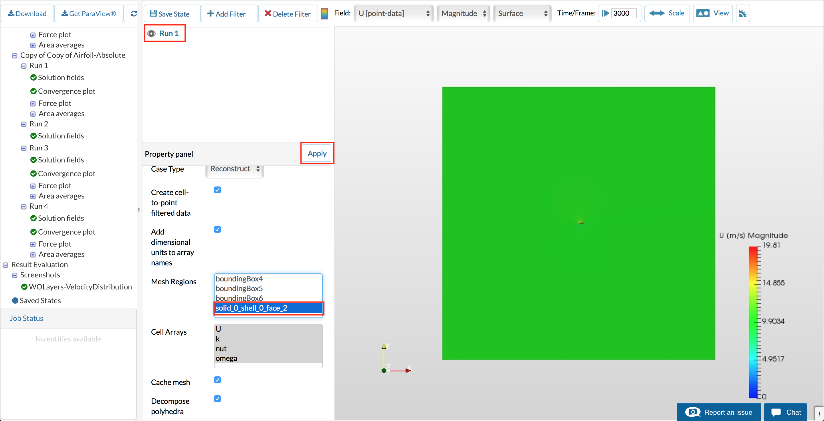
Figure 61: Displaying only Airfoil surface.
Now re-adjust the viewer on the showing surface and change the displayed field to Yplus (Point Data)
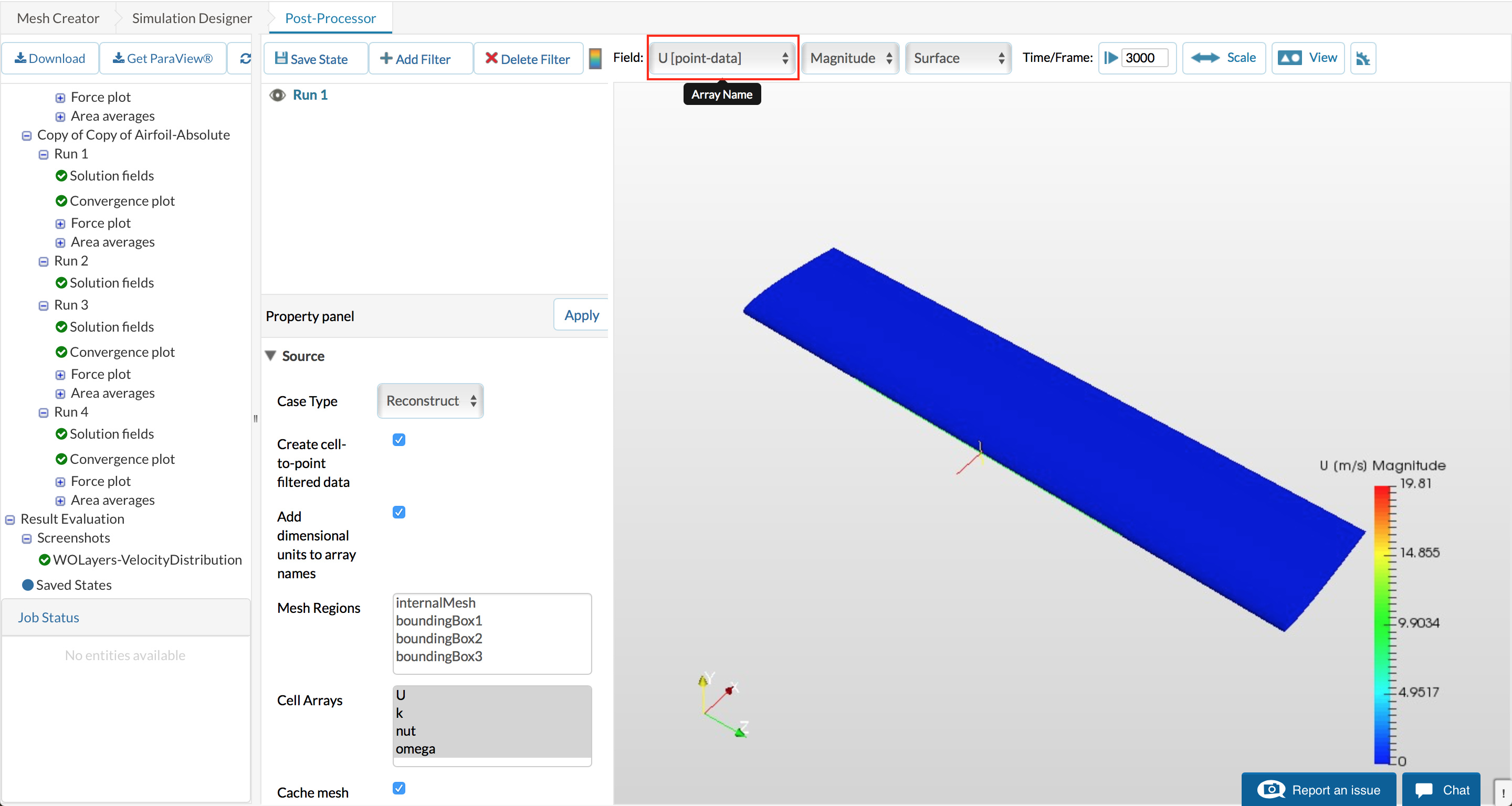
Figure 62: change the displayed field.
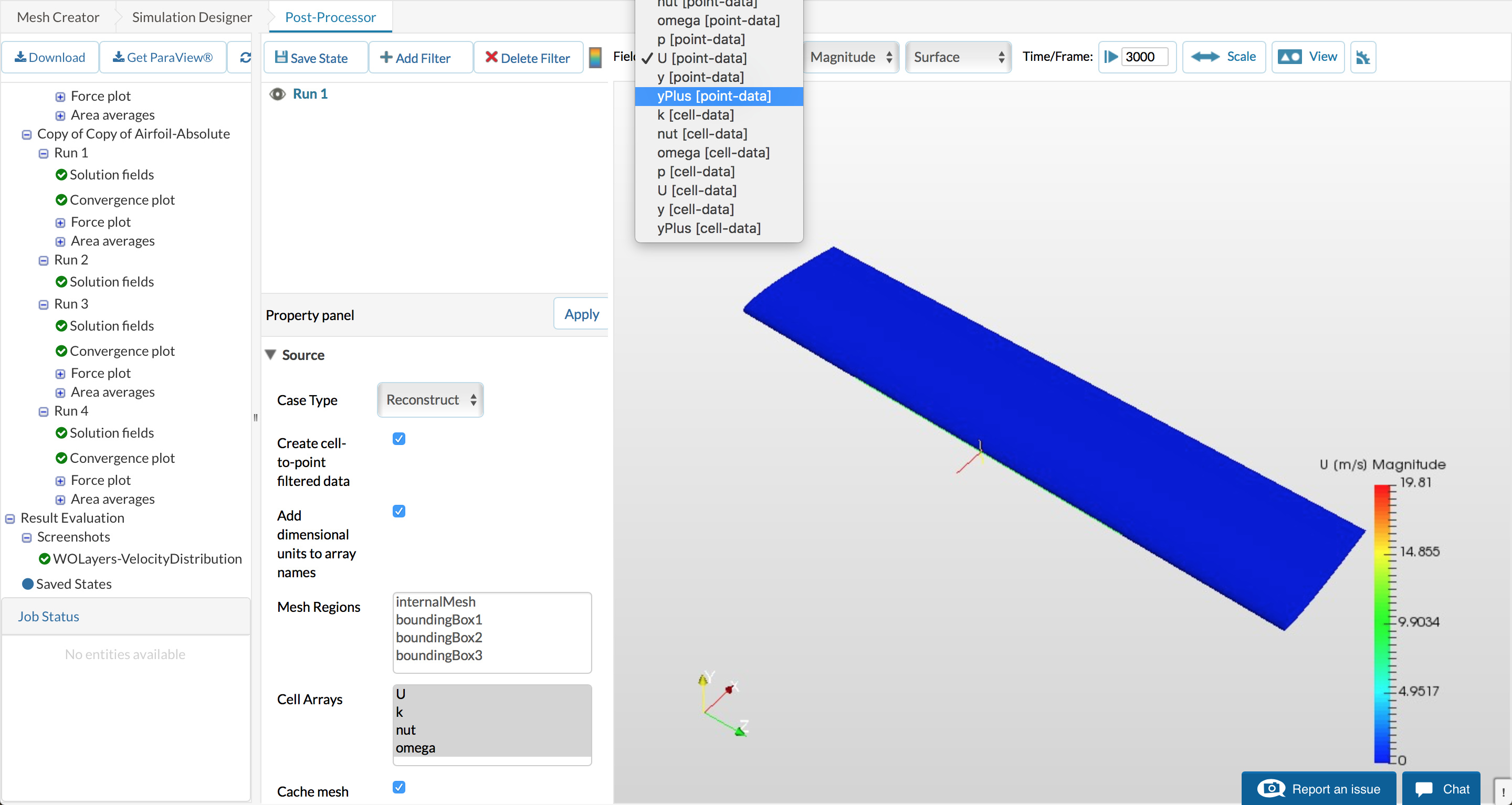
Figure 63: Change the field to Yplus (Point Data).
Change the upper bound scale to 30 (this is the minimum ideal value for the wall function), and enable the legend as we did before. Finally, as before, create a screenshot for later comparison.
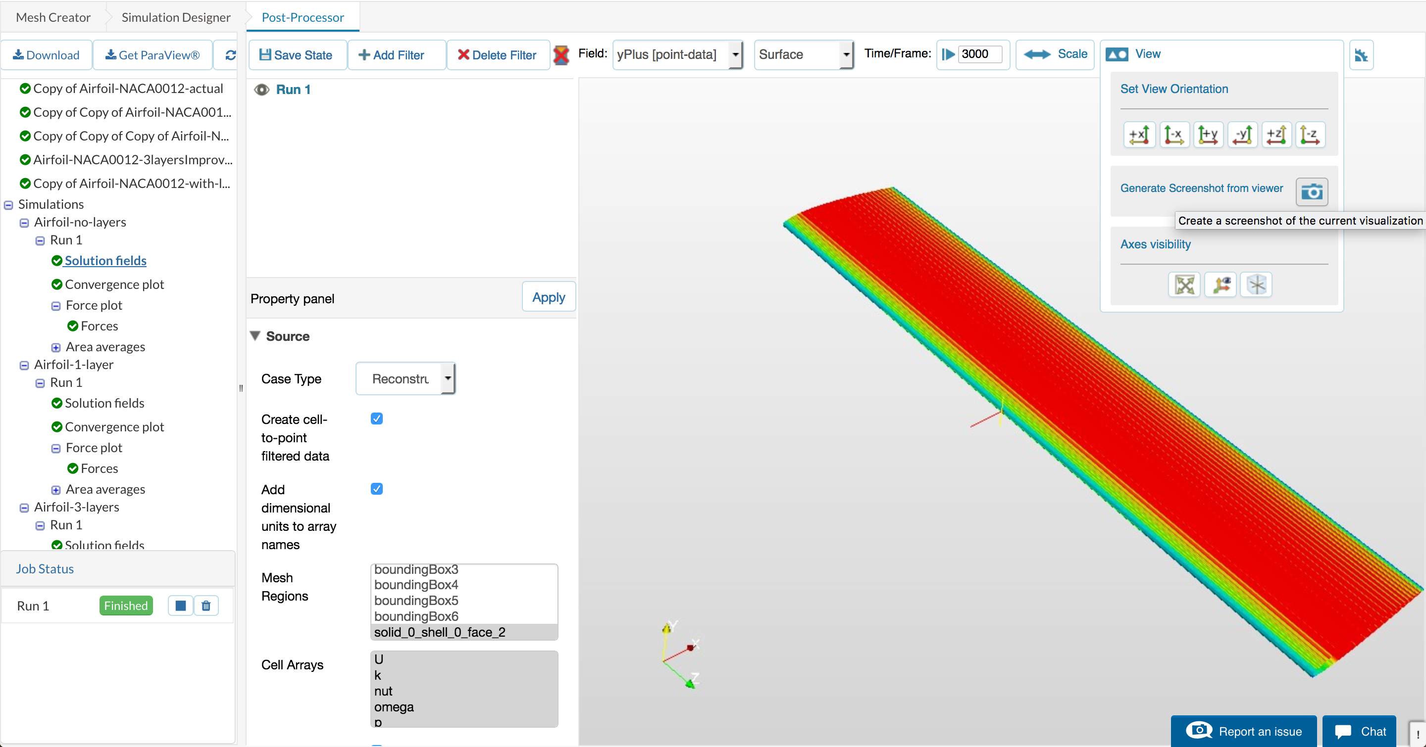
Figure 64: Screenshot of Y+ values.
Change the name of the screenshot to something relevant and repeat this process for the single layer simulation.
Comparing Results
Since the purpose of this exercise is to learn to use and identify the benefits of layer addition at walls for the purpose of wall modelling, we must now compare the results and learn from them. The questions we must ask are;
- How do the velocity profiles compare?
- Which is better?
- Are the Y+ values correct for the modelling technique we are using?
- How can wall distance be modified through changing the mesh?
Starting by tacking the first question should compare the difference between the two velocity profiles.

Looking at these results we observe a significant improvement in smoothness in near-wall velocity, this is due to having parallel cells as opposed to cells being Cartesian orientated. This allows the model to define the velocity on the parallel face and create a gradient between them.
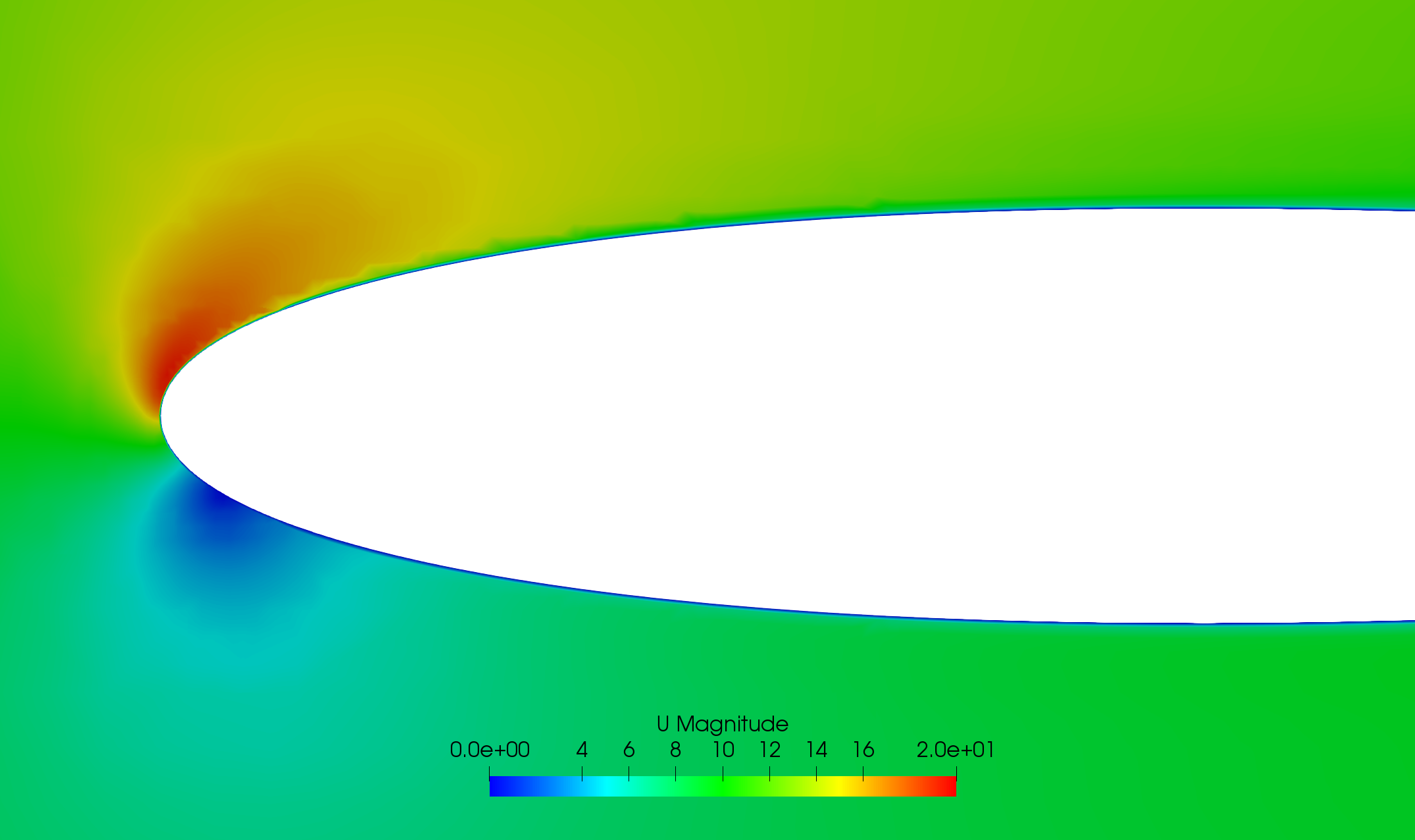
The upper surface leading edge still shows some laddering in velocity after the first cell. This could be improved by adding more layers, and in SimScale the default value is 5 layers. To see the effects of adding more layers to the inflation you can set up a quick mesh and simulation by changing the layer properties to the ones depicted below.
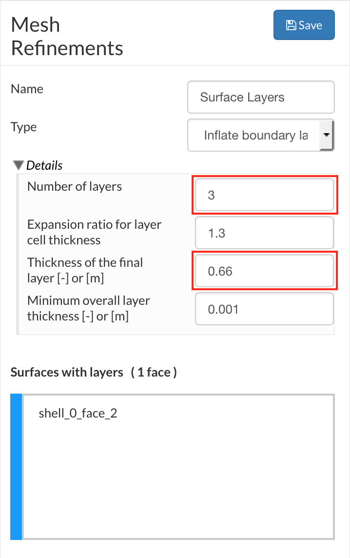
Figure 66: Layer properties for 3 layer inflation.
This produces the better results after the first layer but maintains the same near wall distance.
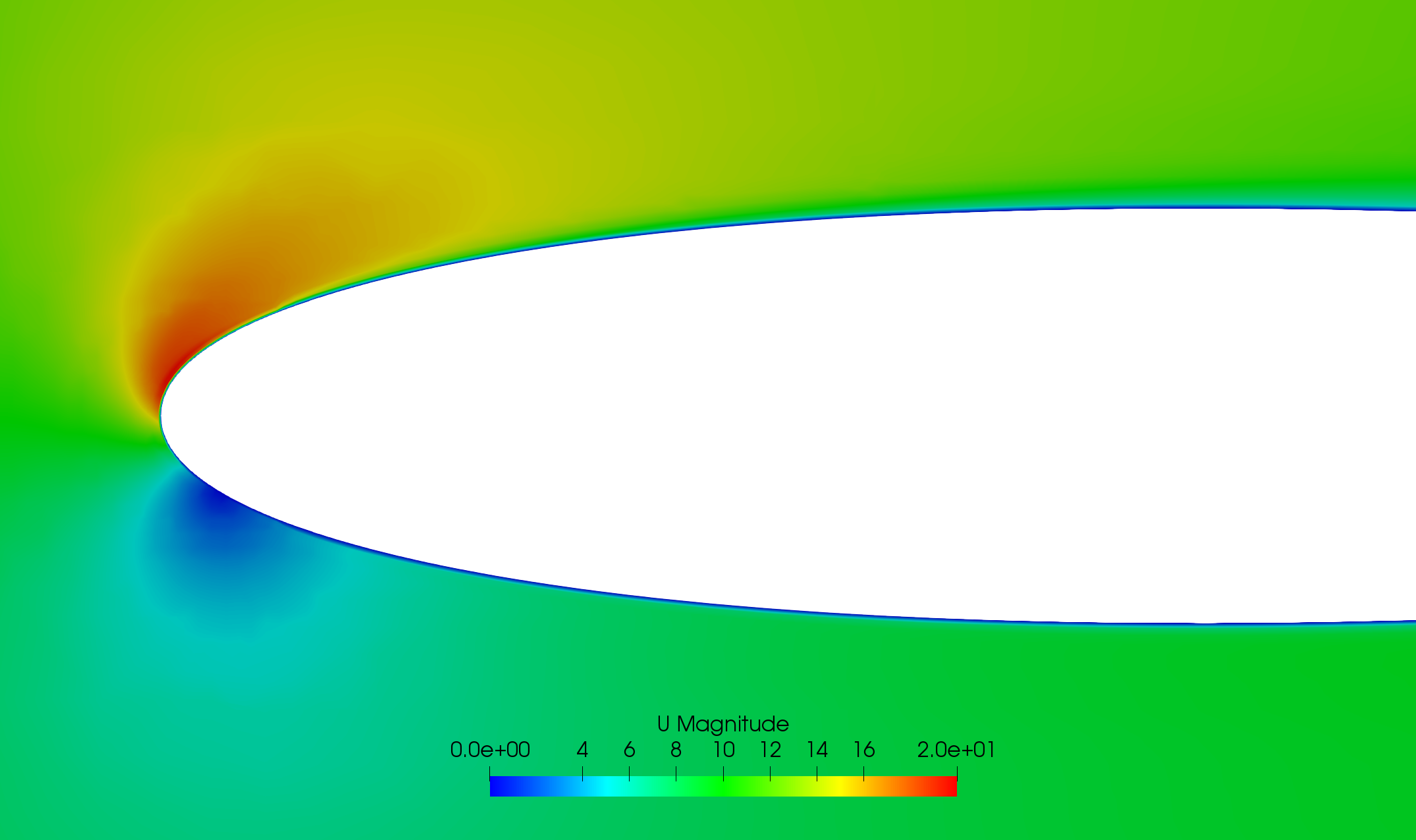
Figure 67: Results from 3 layer inflation.
So we have established that the number of layers effects the velocity profile accuracy and that to a point more layers will improve this profile, however, we now need to consider the thickness of the layer and if it is affecting results. To do this we will look at the post-processing images created earlier.
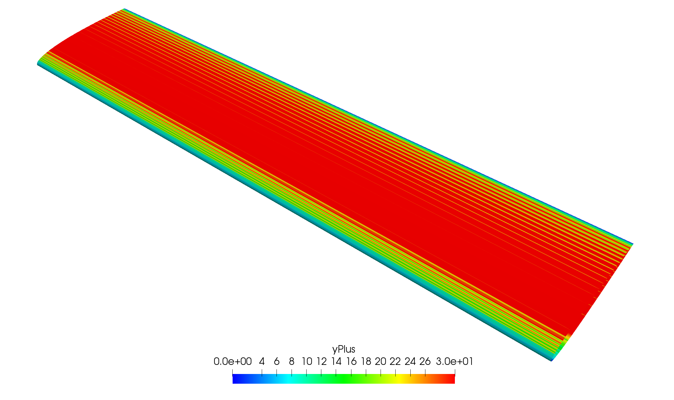
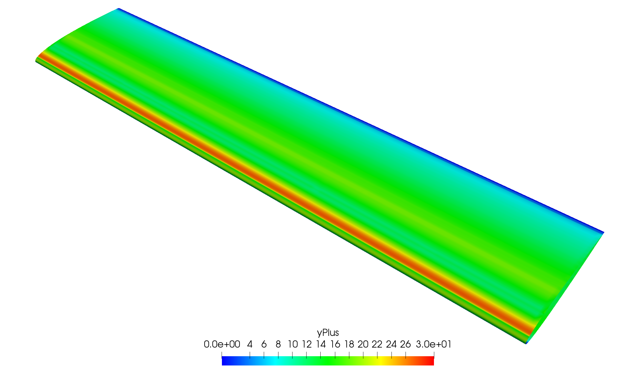
Figure 68: Comparison of first cell Y+ values, no layers (top) and 1 layer (bottom).
Looking t these results we can immediately see that the majority of the y+ values for the mesh with no layers, has a Y+ value in the desired range, however, these values are uneven. This relates to the velocity profile that we saw to also be uneven. In contrast, we can see that the single layer aerofoil has a smooth Y+ value plot but have Y+ values less than desired. This is because the layer is thinner than cells in the no layer mesh.
So we want to have a mesh that does both, it should have a good velocity profile, however, have a majority of the Y+ value to be above 30 (and less than 200). To do this we should increase the size of the layer.
To do this we can simply increase the layer thickness using the following settings.
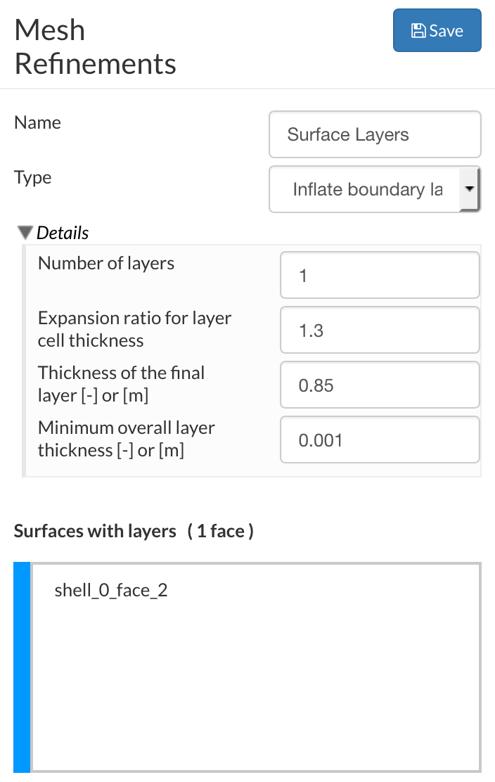
Figure 69: Settings for layer mesh improvement.
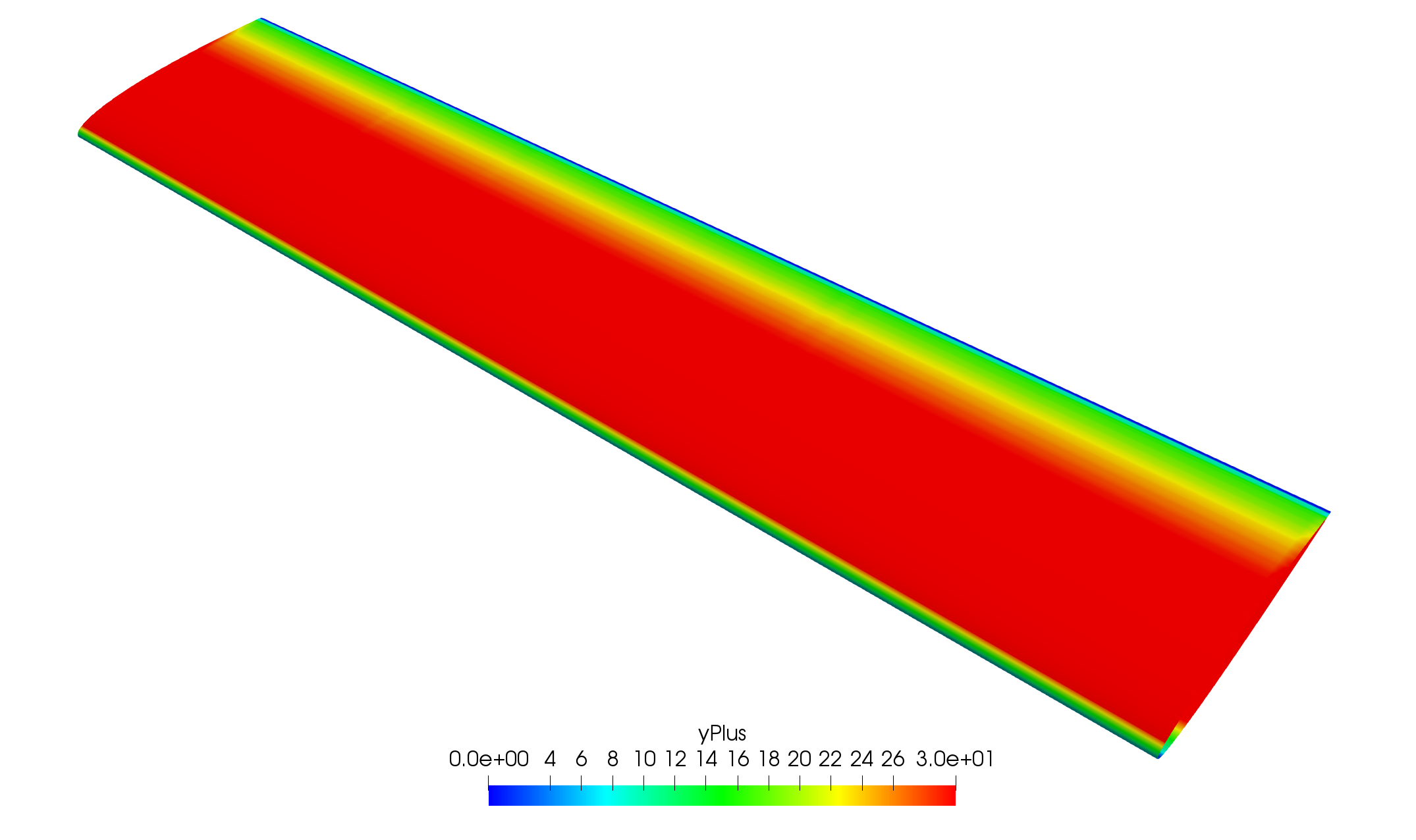
Figure 70: Y+ values of improved layer mesh.
Now we can finally see that the results are not only mostly above 30 but the results are smooth due to the parallel cells along the surface.
What we should consider now, is how much will this affect the result considering the amount of time spent ensuring that the strict requirements are met. To do this we can look at the forces to determine how much physical difference there is. This could also be done using Coefficients if desired.
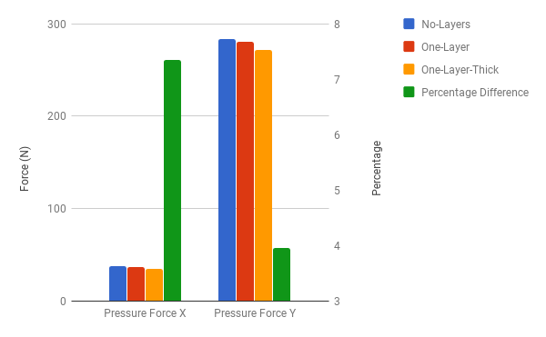
Plot 1: Pressure Forces in the X and Y direction with percentage difference.
From this plot we can see that the difference in results for forces in the x and y-direction are about 7 and 4 percent respectively, this is quite significant and if trying to validate results this could be significant, considering that this is not separated flow which if it was might be affected differently.
